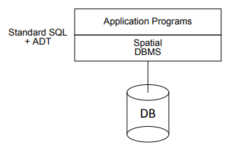
![]()
![]()
Professor: Esteban Zimanyi
Student e-mail: jose.lorencio.abril@ulb.be
This is a summary of the course Advanced Databases taught at the Université Libre de Bruxelles by Professor Esteban Zimanyi in the academic year 22/23. Most of the content of this document is adapted from the course notes by Zimanyi, [1], so I won’t be citing it all the time. Other references will be provided when used.
List of Algorithms
Traditionally, DBMS are passive, meaning that all actions on data result from explicit invocation in application programs. In contrast, active DMBS can perform actions automatically, in response to monitored events, such as updates in the database, certain points in time or defined events which are external to the database.
Integrity constraints are a well-known mechanism that has been used since the early stages of SQL to enhance integrity by imposing constraints to the data. These constraints will only allow modifications to the database that do not violate them. Also, it is common for DBMS to provide mechanisms to store procedures, in the form of precompiled packets that can be invoked by the user. These are usually caled stored procedure.
The active database technology make an abstraction of these two features: the triggers.
Definition 1.1. A trigger or, more generally, an ECA rule, consists of an event, a condition and a set of actions:
Event: indicates when the trigger must be called.
Condition: indicates the checks that must be done after the trigger is called. If the condition is fulfilled, then the set of actions is executed. Otherwise, the trigger does not perform any action.
Actions: performed when the condition is fullfilled.
Example 1.1. A conceptual trigger could be like the following:
| Event | A customer has not paid 3 invoices at the due date. |
| Condition | If the credit limit of the customer is less than 20000€. |
| Action | Cancel all curernt orders of the customer. |
There are several aspects of the semantics of an applications that can be expressed through triggers:
Static constraints: refer to referential integrity, cardinality of relations or value restrictions.
Control, business rules and workflow management rules: refer to restrictions imposed by the business requirements.
Historical data rules: define how historial data has to be treated.
Implementation of generic relationships: with triggers we can define arbitrarily complex relationships.
Derived data rules: refer to the treatment of materialized attributes, materialized views and replicated data.
Access control rules: define which users can access which content and with which permissions.
Monitoring rules: assess performance and resource usage.
The benefits of active technology are:
Simplification of application programs by embedding part of the functionality into the database using triggers.
Increased automation by the automatic execution of triggered actions.
Higher reliability of data because the checks can be more elaborate and the actions to take in each case are precisely defined.
Increased flexibility with the possibility of increasing code reuse and centralization of the data management.
Even though this basic model is simple and intuitive, each vendor proposes its own way to implement triggers, which were not in the SQL-92 standard. We are going to study Starbust triggers, Oracle triggers and DB2 triggers.
Starbust is a Relational DBMS prototype developed by IBM. In Starbust, the triggers are defined with the following definition of their components:
Event: events can refer to data-manipulation operations in SQL, i.e. INSERT, DELETE or UPDATE.
Conditions: are boolean predicates in SQL on the current state of the database after the event has occurred.
Actions: are SQL statements, rule-manipulation statements or the ROLLBACK operation.
Example 2.1. ’The salary of employees is not larger than the salary of the manager of their department.’
The easiest way to maintain this rule is to rollback any action that violates it. This restriction can be broken (if we focus on modifications on the employees only) when a new employee is inserted, when the department of an employee is modified or when the salary of an employee is updated. Thus, a trigger that solves this could have these actions as events, then it can check whether the condition is fullfilled or not. If it is not, then the action can be rollback to the previous state, in which the condition was fullfilled.
The syntax of Starbust’s rule definition is as described in Table 1. As we can see, rules have an unique name and each rule is associated with a single relation. The events are defined to be only database updates, but one rule can have several events defined on the target relation.
The same event can be used in several triggers, so one event can trigger different actions to be executed. For this not to produce an unwanted outcome, it is possible to establish the order in which different triggers must be executed, by using the PRECEDES and FOLLOWS declarations. The order defined by this operators is partial (not all triggers are comparable) and must be acyclic to avoid deadlocks.
Example 2.2. ’If the average salary of employees gets over 100, reduce the salary of all employees by 10%.’
In this case, the condition can be violated when a new employee is inserted, when an employee is deleted or when the salary is updated. Now, the action is not to rollback the operation, but to reduce the salary of every employee by 10%.
First, let’s exemplify the cases in which the condition is violated. Imagine the following initial state of the table Emp:
| Name | Sal |
| John | 50 |
| Mike | 100 |
| Sarah | 120 |
The average salary is 90, so the condition is fullfilled.
INSERT INTO Emp VALUES(’James’, 200)
The average salary would be 117,5 and the condition is not fullfilled.
DELETE FROM Emp WHERE Name=’John’
The average salary would be 110 and the condition is not fullfilled.
UPDATE Emp SET Sal=110 WHERE Name=’John’
The average salary would be 110 and the condition is not fullfilled.
The trigger could be defined as:
Note, nonetheless, that for the first example, we would get the following result:
| Name | Sal |
| John | 45 |
| Mike | 90 |
| Sarah | 108 |
| James | 180 |
Here, the mean is 105.75, still bigger than 100. We will see how to solve this issue later.
At this point, it is interesting to bring some definitions up to scene:
Definition 2.1. A transaction is a sequence of statements that is to be treated as an atomic unit of work for some aspect of the processing, i.e., a transaction either executes from beginning to end, or it does not execute at all.
Definition 2.2. A statement is a part of a transaction, which expresses an operation on the database.
Definition 2.3. En event (in a more precise way than before) is the occurrence of executing a statement, i.e., a request for executing an operation on the database.
Thus, rules are triggered by the execution of operations in statements. In Starbust, rules are statement-level, meaning they are executed once per statement, even for statements that trigger events on several tuples. In addition, the execution mode is deffered. This means that all rules triggered during a transaction are placed in what is called the conflict set (i.e. the set of triggered rules). When the transaction finishes, all rules are executed in triggering order or in the defined order, if there is one. Nonetheless, if the need for a rule executing during a transaction exists, we can use the PROCESS RULES declaration, which executes all rules in the conflict set.
The algorithm for executing all rules after the transaction finished or PROCESS RULES is called is described in Algorithm 1. As we can see, rule processing basically involves 3 stages:
Activation: the event in the rule requests the execution of an operation and this is detected by the system.
Consideration: the condition of the rule is evaluated.
Execution: if the condition is fullfilled, the action in the rule is executed.
As we have seen before, rule definitions specify a partial order for execution, but several rules may have highest priority at the moment of selection. To achieve repeatability, the system maintains a total order, based on the user-defined partial order and the timestamps of the creation of the rules.
Note that the execution of the rules may trigger more rules, this could cause nontermination, if two rules call each other in a cycle. Thus, ensuring termination is one of the main problems of active-rule design.
Example 2.3. Return to the previous example. We saw how the first of the examples did not end up fullfilling the condition, but it is because we did not take into account that the rule would trigger itself because it updates the Salary of Emp. Thus, the insertion and subsequent execution of the rule triggered gave us:
| Name | Sal |
| John | 45 |
| Mike | 90 |
| Sarah | 108 |
| James | 180 |
As we have updated the salaries, the rule is triggered again. The condition would be fullfilled, 105.75>100 and the salaries would be modified again, arriving to the table as:
| Name | Sal |
| John | 41.5 |
| Mike | 81 |
| Sarah | 97.2 |
| James | 162 |
As the salaries ahve been updated again, the rule is triggered once more. Now, the mean is 95.425 < 100, so the condition is not met and the actions are not executed. The rule has terminated.
In this case, termination is ensured because all values are decreased by 10%. This implies that the mean is also decreased by 10%. Thus, no matter how high the mean is at the beginning, at some point it will go below 100, because 0.9x < x, ∀x > 0.
Remark 2.1. In general, guaranteeing termination is responsibility of the programmer is not an easy task.
A transaction causes a state transition of the database, in the form of an addition, suppression of modification of one or more tuples of the database.
Before the transaction commits, the system stores two temporary transition relations, that contain the tuples affected by the transition. This tables are:
INSERTED: for each event, it stores newly inserted tuples and the new form of tuples that have been modified.
DELETED: for each event, it stores deleted tuples and the old form of tuples that have been modified.
Example 2.4. Some simple net effects:
The sequence INSERT → UPDATE → ... → UPDATE → DELETE on a newl tuple, has null effect: the tuple was not in the database at the beginning, and it is not there at the end.
The sequence INSERT → UPDATE → ... → UPDATE on a new tuple, has the same net effect as inserting the tuple with the values given in the last update.
The sequence UPDATE → ... → UPDATE → DELETE on an existing tuple, has the same net effect as just deleting it.
Remark 2.2. Rules consider the net effect of transactions between two database states, so each tuple appears at most once in each temporary table.
Example 2.5. Let’s see the INSERTED and DELETED tables of our example. We start with the table
| Name | Sal |
| John | 50 |
| Mike | 100 |
| Sarah | 120 |
And perform UPDATE Emp SET Sal=110 WHERE Name=’John’. If we accessed the temporary tables now, we would see:
| INSERTED | |
| Name | Sal |
| John | 110 |
| DELETED | |
| Name | Sal |
| John | 50 |
Now, the rule is triggered because salary has been updated. The condition is met and the action is launched. If we accessed the temporary tables now, we would see:
| INSERTED | |
| Name | Sal |
| John | 99 |
| Mike | 90 |
| Sarah | 108 |
| DELETED | |
| Name | Sal |
| John | 50 |
| Mike | 100 |
| Sarah | 120 |
Note how the first tuple in INSERTED shows only the net effect on the tuple.
With this definitions, we can give a more precise definition of rule triggering:
A great feature of rules is that it is possible to reference the transition tables, which can be very useful in many occasions.
Example 2.6. Now, imagine we want to add the rule ’If an employee is inserted with a salary greater than 100, add the employee to the table of hifh paid employees’. This rule could be defined as:
When we insert (James, 200), the tuple is inserted and the rules SalaryControl and HighPaid are triggered. Because we have defined HighPaid to follow SalaryControl, the latter would execute earlier. Now, SalaryControl, as we saw, would trigger more instances of the same rule, which would be all executed before HighPaid. At the end, as all employees would have been modified, all of them with a salary bigger than 100 would be added to the table HighPaidEmp because of this new rule. In this case, only James fullfills the condition.
In Oracle, the term used is TRIGGER. Triggers in Oracle respond to modification operations (INSERT, DELETE, UPDATE) to a relation, just as in Starburst.
The triggers in Oracle can be defined for different granularities:
Tuple-level: the rule is triggered once for each tuple concerned by the triggering event.
Statement-level: the rule is triggered only once even if several tuples are involved.
Also, the execution mode of triggers in Oracle is immediate, meaning they are executed just after the event has ben requested, in contrast to Starburst, in which the execution mode is referred, as we saw. This allows for rules to be executed before, after or even instead of the operation of the triggering event. In 3, the definition syntax of triggers in Oracle is detailed. Some notes:
The BEFORE or AFTER commands define when the rule should execute in relation to the events that trigger it.
If FOR EACH ROW is written, then the trigger is a tuple-level trigger, and it is activated once for each tuple concerned.
This is useful if the code in the actions depends on data provided by the triggering statement or on the tuples affected.
The INSERTING, DELETING and UPDATING statements may be used in the action to check which triggering event has occurred.
OLD and NEW reference the old value of the tuple (if it is update or delete) and the new value of the tuple (if it is update or insert).
The condition consists of a simple predicate on the current tuple.
If FOR EACH ROW is not written, then the trigger is a statement-level trigger, and it is activated once for each triggering statement even if several tuples are involved or no tuple is updated.
Oracle triggers can execute actions containing arbitrary PL/SQL2 code (not just SQL as in Starburst).
Example 2.7. Row-level AFTER trigger.
Imagine we have two tables:
Inventory(Part, PartOnHand, ReorderPoint, ReorderQty)
PendingOrders(Part, Qty, Date)
We want to define a rule that whenever a PartOnHand is modified, and its new value is smaller than the ReorderPoint (i.e. we have less parts than the threshold to order more parts), we add a new record to PendingOrders as a new order for this part and the required quantity, if it is not already done. This can be done as follows:
Let’s apply the rule to see how it works. Let’s say our table Inventory is:
| Part | PartOnHand | ReorderPoint | ReorderQty |
| 1 | 200 | 150 | 100 |
| 2 | 780 | 500 | 200 |
| 3 | 450 | 400 | 120 |
If we execute the following transaction on October 10, 2000:
Then the tuple (1,100,2000-10-10) would be inserted into PendingOrders.
The algorithm for executing rules in Oracle is shown in Algorithm 2. As we can see, statement-level triggers are executed before/after anything else, and row-level triggers are executed before/after each affected tuple is modified. Note that the executions needs to take into account the priority among triggers, but only those of the same granularity (row vs statement) and type (before vs after).
The action part may activate other triggers. In that case, the execution of the current trigger is suspended and the others are considered using the same algorithm. There a maximum number of cascading triggerss, set at 32. When this maximum is reached, execution is suspended and an exception is raised.
If an exception is raised or an error occurs, the changes made by the triggering statement and the actions performed by triggers are rolled back. This means that Oracle supports partial rollback instead of transaction rollback.
This is another type of Oracle trigger, in which the action is carried out inplace of the statement that produced the activating event. These triggers are typically used to update views and they need to be carefully used, because changing one action Y for an action X can sometimes have unexpected behaviors.
Example 2.8. An Instead-of trigger:
This trigger automatically updates the manager of a department when a new manager is inserted.
In DB2, every trigger monitors a single event, and are activated immediately, BEFORE or AFTER their event. They can be defined row-level or statement-level, as in Oracle. But in this case state-transition values can be accessed in both granularities:
OLD and NEW refer to tuple granularity, as in Oracle.
OLD_TABLE and NEW_TABLE refer to table granularity, like the DELETED and INSERTED in Starburst.
DB2’s triggers cannot execute data definition nor transactional commands. They can raise errors which in turn can cause statement-level rollbacks.
The syntax is as in Table 4.
The processing is done as in Algorithm 3. Note that:
Steps 1) and 6) are not required when S if part of an user transaction.
If an error occurs during the chain processing of S, then the prior DB state is restored.
IC refers to Integrity Constraints.
Before-triggers: these are used to detect error conditions and to condition input values. They are executed entirely before the associated event and they cannot modify the DB (to avoid recursively activating more triggers).
After-triggers: these are used to embed part of the application logic in the DB. The condition is evaluated and the action is possibly executed after the event occurs. The state of the DB prior to the event can be reconstructed from transition values.
Several triggers can monitor the same event.
In this case, the order is total and entirely based on the creation time of the triggers. Row-level and statement-level triggers are intertwined in the total order.
If the action of a row-level trigger has several statements, they are all executed for one tuple before considering the next one.
Example 2.9. Imagine we have the following two tables:
| Part | ||
| PartNum | Supplier | Cost |
| 1 | Jones | 150 |
| 2 | Taylor | 500 |
| 3 | HDD | 400 |
| 4 | Jones | 800 |
| Distributor | ||
| Name | City | State |
| Jones | Palo Alto | CA |
| Taylor | Minneapolis | MN |
| HDD | Atlanta | GA |
And there is a referential integrity constraint that requires Part Suppliers to be also distributors, with HDD as a default Supplier:
Then, the following trigger is a row-level trigger that rollbacks when updating Supplier to NULL:
In SQL Server, a single trigger can run multiple actions, and it can be fired by more than one event. Also, triggers can be attached to tables or views. SQL Server does not support BEFORE-triggers, but it supports AFTER-triggers (they can be defined using the word AFTER or FOR3 ) and INSTEAD OF-triggers.
The triggers can be fired with INSERT, UPDATE and DELETE statements.
The option WITH ENCRYPTION encrypts the text of the trigger in the syscomment table.
Finally, the option NOT FOR REPLICATION ensures that the trigger is not executed when a replication process modifies the table to which the trigger is attached.
The syntax is shown in Table 5.
INSTEAD OF-triggers: are defined on a table or a view. Triggers defined on a view extend the types of updates that a view support by default. Only one per triggering action is allowed on a table or view. Note that views can be defined on other views, and each of them can have its own INSTEAD OF-triggers.
AFTER-triggers: are defined on a table. Modifications to views in which the table data is modified in response, will fire the AFTER-triggers of the table. More than one is allowed on a table. The order of execution can be defined using the sp_settriggerorder procedure. All other triggers applied to a table execute in random order.
Both clases of triggers can be applied to a table.
If both trigger classes and constraints are defined for a table, the INSTEAD OF-trigger fires first. Then, constraints are processed and finally AFTER-triggers are fired.
If constraints are violated, INSTEAD OF-trigger’s actions are rolled back.
AFTER-triggers do not execute if constraints are violated or if some other event causes the table modification to fail.
As stored procedures, triggers can be nested up to 32 levels deep and fired recursively.
Two transition tables are available: INSERTED and DELETED, which are as in Starburst.
The IF UPDATE(<column-name> clause determines whether an INSERT or UPDATE event ocurred to the column.
The COLUMNS_UPDATE() clause returns a bit pattern indicating fhich of the tested columns were isnerted or updated.
The @@ROWCOUNT function returns the number of rows affected by the previous Transact-SQL statement in the trigger.
A trigger fires even if no rows are affected by the event. The RETURN command can be used to exit the trigger transparently when this happens.
The RAISERROR command is used to display error messages.
There are some Transact-SQL statements that are not allowd in triggers:
ALTER, CREATE, DROP, RESTORE and LOAD DATABASE.
LOAD and RESTORE LOG.
DISK RESIZE and DISK INIT.
RECONFIGURE.
If in a trigger’s code it is needed to assign variables, then SET NOCOUNT ON must be included in the trigger code, disallowing the messages stating how many tuples were modified in each operation.
The INSTEAD OF DELETE and INSTEAD OF UPDATE triggers cannot be defined on tables that have a correspoonding ON DELETE or ON UPDATE cascading referential integrity defined.
Triggers cannot be created on a temporary or system table, but they can be referenced inside other triggers.
SQL Server enables to enable or disable nested and recursive triggers:
Nested trigger option: determines whether a trigger can be executed in cascade. There is a limit of 32 nested trigger operations. It can be set with sp_configure ’nested triggers’, 1 | 0.
Recursive trigger option: causes triggers to be re-fired when the trigger modifies the same table as it is attached to: the neste trigger option must be set to true. This option can be set with sp_dboption ’<db-name>’, ’recursive triggers’, ’TRUE’ | ’FALSE’.
Note that recursion can be direct if a trigger activates another instance of itself or indirect if the activation sequence is T1 → T2 → T1. The recursive trigger option only copes with the direct recursion, the indirect kind is dealt with the nested trigger option.
Trigger management includes the task of altering, renaming, viewing, dropping and disabling triggers:
Triggers can be modified with the ALTER TRIGGER statement, in which the new definition is provided.
Triggers can be renamed with the sp_rename system stored procedure as
sp_rename @objname = <old-name>, @newname = <new-name>
Triggers can be viewed by querying system tables or by using the sp_helptrigger and sp_helptext system stored procedures as
sp_helptrigger @tabname = <table-name>
sp_helptext @objname = <trigger-name>
Triggers can be deleted with the DROP TRIGGER statement.
Triggers can be enable and disable using the ENABLE TRIGGER and DISABLE TRIGGER clauses of the ALTER TABLE statement.
Example 2.10. Let’s work with a database with the following tables:
Books(TitleID, Title, Publisher, PubDate, Edition, Cost, QtySold)
Orders(OrderId, CustomerId, Amount, OrderDate)
BookOrders(OrderID, TitleId, Qty)
Here, Books.QtySold is a derived attribute which keeps track of how many copies of the book has been sold. We can make this updates automatic with the use of the following trigger:
When there is an insertion in BookOrders, the trigger fires and adds the corresponding quantity.
When there is a deletion, the trigger fires and subtracts the corresponding quantity.
An update creates both tables, so we would add and subtract to cope with the modification.
Rules provide programmers with an effective tool to support both internal applications and external applications:
Internal applications: rules support function provided by specific subsystems in passive DBSMs, such as the management of IC, derived data, replicated data, version maintenance,... Rules can usually be declaratively specified, generated by the system and hidden to the user.
External applications: these refer to the application of business rules to the data stored. Rules allow to perform computations that would usually need to be expressed in application code. In addition, rules provide many times a natural way to model reactive behavior of the data, as rules respond to external events and perform action in consequence. This approach becomes specially interested when rules express central policies, i.e., knowledge common to applications, centralizing the effort and reducing the cost.
Some examples of applications that can benefit from active technology and business rules are:
Monitoring access to a building and reacting to abnormal circumstances.
Watching evolution of share values on stock market and triggering trading actions.
Managing inventory to follow stock variations.
Managing a netwrok to for energy distribution.
Airway assignment in air traffic control.
As can be seen from these examples, a frequent case of application-specific rules are alterters, whose actions signal certain conditions that occur with ot without changing the database.
The integrity of a database refers to the consistency and conformity of the data with the database schema and its constraints. Thus, an integrity constraint is any assertion on the schema which is not defined in the data-structure aprt of the schema. Constraints declaratively specify conditions to be satisfied by the data at all times, so checking for integrity violations is done for every update of the state of the database.
Integrity constraints can be static if the predicates are evaluated on database states or dynamic if the predicates are evaluated on state transitions. They can also be classified as built-in if they are defined by special DDL (Data Definition Language) constructs (such as keys, nonnull values,...) or adhoc, which are arbitrarily complex domain-dependent constraints.
In practice, integrity maintenance is achieved through:
DBMS checks built-in constraint with automatically generated triggers.
DBMS supports limited forms of adhoc constraints.
The remaining constraints are implemented as active rules (triggers).
The process of rule generation may be partially automated:
The possible causes of violation are the events for the activation of the rule.
The declarative formulation of the constraint is the rule condition.
To avoid or eliminate the violation, an action is taken. The simplest approach is to rollback the transaction, this is done by abort rules, in contrast, the richer approach provides a domain-dependent corrective action, via repair rules.
Thus:
Abort rules check that integrity is not violation and prevent the execution of an operation which would cause the violation of the integrity by means of the ROLLBACK command.
Repair rules are more sophisticated than abort rules, because they make use of application-domain semantics to define a set of actions that restore integrity
Example 3.1. Let’s do a referential integrity example in Starburst:
We have relations Emp(EmpNo,DeptNo) and Dept(DNo). We have the regerential integrity condition
![Emp [DeptN o] ⊂ Dept[DN o],](summary0x.png)
so the possible violations can come from an INSERT into Emp, a DELETE from Dept, and UPDATE of Emp[DeptNo] and an update of Dept[Dno]. The condition on tuples of Emp for not violating the constraint is:
Its denial form, so the constraint is violated is:
Thus, we can create abort rules as:
Note that one rule is neccessary for each relation.
Note also that the defined rules are inneficient, because the computation of the condition checks the whole database. Rules can assume that the constraint is verified in the initial state, so it suffices to compute the condition relative to transition tables.
Now, we are defining a repair rule that:
If an employee is inserted with a wrong value of DeptNo, it is set to NULL.
If the DeptNo of an employee is updated with a wrong value of DeptNo, it is set to 99.
If a department is deleted or its DNo is updated, then all employees from this department are deleted.
A view can be seen as a query on the DB which returns a relation or a class that can be used as any other relation or class. A derived attribute is an attribute that can be computed from other attributes in the DB. Both a view and a derived attribute can be expressed with declarative query language or deductive rules. There are two strategies for derived data:
Virtually supported: their content is computed on demand.
Materialized: their content is stored in the database, and it must be recomputed whenever the source of data is changed.
When an application queries a view, a rule is triggered on the request and the action substitutes and evaluates the view definition. It requires an event, triggered by queries, and an INSTEAD OF clause in rule language.
There exist two basic strategies:
Refresh: recompute the view from scratch after each update of the source data.
Incremental: compute changes to the view from changes in the source relations, using positive and negative deltas (a delta shows the changes experienced in the database. INSERTED and DELETED are one way to implement deltas).
The rule generation can be automated. Refresh rules are simple, but can be very inefficient. On the other hand, incremental rules depend on the structure of derivation rules, and can be complex.
Example 3.2. Imagine we have the following view definition:
So this view holds are departments in which some employee earns more than 50k€ a year. This view can change whenever an employee is inserted or deleted, its department is changed or is salary is changed; and whenever a department is inserted or deleted, or its Dno is updated.
A refresh rule defined in Starburst to handle this changes is:
As we can see, all elements from the view are deleted, and the view is recomputed entirely. The incremental approach is more complex. As an example, let’s define the rule for the case of Insert Dept:
Replication consists on storing several copies of the same information. This is a common practice in distributed databases. Keeping fully synchronized copies is usually very costly and unnecessary, so it is common to use aynchronous techniques to propagate changes between nodes.
Assymmetric replication: in this case there exists a primary copy, in which changes are performed, and several secondary copies, which are read only and are updated asynchronously. The capture module monitors changes made by applications to the primary copy, and the application module propagates these changes to the secondary copies.
Symmetric replication: all copies accept updates asynchronously and each of them has a capture and an application modules. It is needed to be careful, because simultaneous updates may cause loss of consistency.
Example 3.3. An example of capturing changes into deltas in Starburst:
The deltas are applied to the copies with a predefined policy, e.g. once very hour.
Active rules can impose a central consistent behavior independent of the transactions that cause their execution.
Active rules enforce data management policies that no transaction can violate.
Activities redundantly coded in several applications programs with passive DBMSs can be abstracted in a single version as a rule in an active DBMS.
Data management policies can evolve by just modifying the rules on the database, instead of the application programs (knowledge independence).
Rule organization and content are often hard to control and to specify declaratively (i.e. the rules are hard to code!).
Understanding active rules can be difficult, because they can react to intricate event sequences and the outcome of rule processing can depend on the order of the event ocurrences and the rule scheduling, which can be hard to analyze in complex systems.
There are no easy-to-use nor one-fits-all techniques for designing, debugging, verifying and monitoring rules.
This is an example of an application modeled with active rules, covering the business process:
’Management of the Italian electrical power distribution network.’
The operational network is a forest of trees, connecting power distributors to users. The operating conditions are monitored constantly with frequent reconfigurations: the structure of the network is dynamic. The topology is modified less frequently (we can consider it static). The objective is to transfer the exact power from distributors to users through nodes and directed branches connecting pairs of nodes.
In this scenario, active rules are used to respond to input transactions asking for:
Reconfigurations due to new users.
Changes in their required power.
Changes in the assignment of wires.
The schema of the database is:
BranchIn, Power) foreign key (BranchIn) References Branch
FromNode, ToNode, Power)
BranchIn, Power) foreign key (BranchIn) References Branch
Power, MaxPower)
BranchId, WireType, Power) foreign key (BranchId) references Branch foreign key (WirteType) references WireType
MaxPower)
The network is composed of sites anc onnections between pairs of sites:
Sites comprise:
Power stations: distributors where power is generated and fed into the network.
Intermediate nodes: nodes where power is transferred to be redistributed across the network.
Final users of electrical power.
Connections are called branches:
class Branch describes all connections between pairs of sites.
Several Wires are placed along the branches.
Wires are made of a given WireType, each type carrying a maximum power.
Branches can be dinamically added or dropeed to the network.
The business rules are the following:
Several user requests are gathered in a transaction.
If the power requested on wires excees the maximum power of the wire type, rules change or add wires in the relevant branches.
Rules propagate changes up in the tree, adapting the network to new user needs.
A transaction fails if the maximum power requested from some distributor exceeds the maximum power available at the distributor (in that case, the static network needs to be redesigned, but this is out of our scope).
To avoid unnecessary rollbacks, rules propagate reductions of power first, then increases of power. This requires setting the order in which the triggers execute4 .
A new user is connecting to a node with the following procedure:
The node to which a user is connected is determined by an external application: usually its closest node. ’WT1’ is the basic wire type. nextUserId, nextBranchId and nextWireId procedures are used to obtain the next identifier of a user, branch or wire.
If a user requires less power, this change needs to be propagated to its input branch:
If a node require less power, propagate the change to its input branch:
If a branch connected to a node requires less power, propagate the change to its input node.
If a branch connected to a distributor requires less power, propagate the change to the distributor.
If a user requires more power, propagate the change to its input branch.
If a node require more power, propagate the change to its input branch:
If a branch connected to a node requires more power, propagate the change to its input node.
If a branch connected to a distributor requires more power, propagate the change to the distributor.
If the power requested from a distributor exceeds its maximum, rollback the entire transaction.
If the power of a branch is changed, distributes the change equally on its wires.
If the power on a wire goes above the allowed threshold, change the wire type.
If there is no suitable wire type, add another wire to the branch.
Relational DBMSs are too rigid for Big Data scenarios, and not the best option for storing unstructured data. The one-size-fits-all approach is no longer valid in many scenarios and RDBMSs are hard to scale for billions of rows, because data structures used in RDBMSs are optimized for systems with small amounts of memory.
NoSQL technologies do not use the relational model for storing data nor retrieving it. Also, they don’t generally have the concept of schema, so fields can be added to any record as desired, without control. These characteristics provide ease to run on clusters as well as an increased scaling capability, with horizontal scalability in mind. But these gains are not free: there is a trade-off in which the traditional concept of consistency gets harmed. For example, ACID (Atomic, Consistent, Isolated, Durable) transactions are not fully supported most of the times.
There are several types of NoSQL databases, such as Key-Value stores, Column stores, Document databases,... We are going to focus on Graph Databases.
Definition 4.1. The consistency of a database is fullfilled when all updates happen equally for all users of the database.
The availability guarantees that every request receives a response, whether it succeeded or failed.
The partition tolerance means that the system is able to operate despite arbitrary message lost or failure of part of the system.
A database has, ideally, this three properties fullfilled. But the CAP theorem ensures that this is impossible:
Remark 4.1. If the system needs to be distributed, then partition tolerance is a must. So, in practice, there is a decision to choose between fullfilling consistency or availability for distributed systems.
Remark 4.2. Nonetheless, even the perfect form of the three properties cannot be guaranteed at once, it is possible to provide fairly good levels of the one that is not optimal.
With fewer replicas in the system, R/W operations complete more quickly, improving latency.
In graph databases, the data and/or the schema are represented by graphs, or by data structures that generalize the notion of graph: hypergraphs.
The integrity constraints enforce data consistency. Constraints can be grouped in: schema-instance consistency, identity and referencial integrity, and functional and inclusion dependencies.
The data manipulation is expressed by graph transfromations, or by operations whose main primitives are on graph features, like paths, neighborhoods, subgraphs, connectivity and graph statistics.
RDF allows to express facts, such as ’Ana is the mother of Julia.’, but we’d like to be able to express more generic knowledge, like ’If somebody has a daughter, then that person is a parent.’. This kind of knowledge is called schema knowledge. The RDF schema allows us to do some schema knowledge modeling, and the Ontology Web Language (OWL) gives even more expressivity.
A class is a set of things or resources. In RDF, everything is a resource, that belongs to a class (or several classes). The classes can be arranged in hierarchies. Every resource is a member of the class rdfs:Class.
The different resources are labelled with:
rdfs:Resource: class of all resources.
rdf:Property: class of all properties.
rdfs:XMLLiteral: class of XML resources.
rdfs:Literal: each datatype is a subclass.
rdfs:Bag, rdf:Alt, rdf:Seq, rdfs:Container, rdf:List, rdf:nil, rdfs:ContainerMembershipProperty.
rdfs:Datatype: class of all datatypes.
rdfs:Statement.
In RDF, there exists implicit knowledge, which can be inferred using deduction. This knowledge doesn’t need to be stated explicitly: which statements are logical consequences from others is governed by the formal semantics.
Example 4.2. If a RDF document contains ’u rdf:type ex:Textbook’ and ’ex:Textbook rdfs:subClassOf ex:Book’, then it is deduced that ’u rdf:type ex:Book’.
As can be seen, RDF are usually stored in triple stores or quad stores, which are a relational DB. This means that it is usually not implemented natively as a graph database, which makes it harder to do inference. It is more usually used as a metadata storage.
This model is simpler: in this case, the model is a graph, where nodes and edges are annotated with properties. It is schema-less, meaning there is not an underlying schema to which the data has to adhere. Inference is not performed.
There are several types of relationships supported by graph databases:
Attributes: properties that can be uni- or multi- valued.
Entities: groups of real-world objects.
Neighborhood relations: structures to represents neighborhoods of an entity.
Standard abstractions: part-of, composed-by, n-ary associations.
Derivation and inheritance: subclasses and superclasses, relations of instantiations.
Nested relations: recursively specified relations.
The abstract data type used is a graph with properties, which is a 4-tuple G =  such that:
V is a finite set of nodes.
Σ is a set of labels.
E ⊂ V × V is a set of edges representing labelled binary relationships between elements in V .
L is a function, L : V ×V → 2Σ, meaning that each edge can by annotated with zero or more labels from Σ.
The basic operations defined over a graph are:
AddNode : adds node x to G.
DeleteNode : deletes x from G.
Adjacent : tests if there is an edge from x to y in G, i.e., if
  ∈ E.
∈ E.
Neighbors : returns all nodes y such that
  ∈ E.
∈ E.
AdjacentEdges : returns the set of lables of edges going from x to y.
Add : adds an edge between x and y with label l.
Delete : deletes and edge between x and y with label l.
Reach : tests if there is a path from x to y. A path between x and y is a subset of nodes z1,...,zn
such that
: tests if there is a path from x to y. A path between x and y is a subset of nodes z1,...,zn
such that  ,
, ∈ E and
  ∈ E for all i = 1,...,n - 1. The length of the path is how
many edges there are from x to y.
∈ E for all i = 1,...,n - 1. The length of the path is how
many edges there are from x to y.
Path : return a shorthest path from x to y.
2 - hop : return the set of nodes that can be reached from x using paths of length 2.
n - hop : returns the set of ndoes that can be reached from x using paths of length n.
The notion of graph can be generalized by that of hypergraph, which is a pair H =  , where V is a set of nodes, and
E ⊂ 2V is a set of non-empty subsets of V , called hyperedges. If V =
, where V is a set of nodes, and
E ⊂ 2V is a set of non-empty subsets of V , called hyperedges. If V =  and E =
  , we can define
the incidence matrix of H as the matrix A =
, we can define
the incidence matrix of H as the matrix A =  n×m where
In this case, this is an undirected hypergraph. A directed hypergraph is defined similarly by H =  where in this case E ⊂ 2V × 2V , meaning that the nodes in the left set are connected to the nodes of the right
one.
where in this case E ⊂ 2V × 2V , meaning that the nodes in the left set are connected to the nodes of the right
one.
In an adjacency list, we maintain an array with as many cells as there are nodes in the graph, and:
For each node, maintain a list of neighbors.
If the graph is directed, the list is only containing outgoing nodes.
This way it is very cheap to obtain neighbors of a node, but it is not suitable for checking if there is an edge between two nodes.
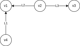
Is modelled with the following adjacency list:
| v1 | |
| v2 | {(v1,{L2}),(v3,{L4})} |
| v3 | |
| v4 | {(v1,{L1})} |
In this case, we maintain two arrays, one with as many cells as nodes, and another one with as many different edges there are in the graph:
Vertices and edges are stored as records of objects.
Each vertex stores incident edges, labeled as source if the edge goes out, or destination if it goes in.
Each edge stores incident nodes.
Example 4.4. Now, the graph of the previous example is modeled as:
| v1 | {(dest,L2),(dest,L1)} |
| v2 | {(source,L2),(source,L3)} |
| v3 | {(dest,L3)} |
| v4 | {(source,L1)} |
| L1 | (V4,V1) |
| L2 | (V2,V1) |
| L3 | (V2,V3) |
Some properties:
Storage is O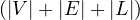 .
.
Adjacent is O
is O , we have to check at most all edges.
Neighbors is O
is O , we go to node x and for each edge marked as source, we visit it and return
the correspondant destination. At most E checks.
, we go to node x and for each edge marked as source, we visit it and return
the correspondant destination. At most E checks.
AdjacentEdges is again O
 .
.
Add is O
is O , as well as delete Delete
 .
.
In this case, we maintain a matrix of size n × n, where n is the number of nodes:
It is a bidimensional graph representation.
Rows represents source nodes.
Columnds represent destination nodes.
Each non-null entry represents that there is an edge from the source node to the destination node.
Properties:
The storage is O .
.
Adjacent is O
is O , we have to check cell
  .
.
Compute the out-degree of a node is O , we have to sum its row.
For the in-degree it is also O , we have to sum its column.
Adding an edge between two nodes is O .
.
Compute all paths of length 4 between any pair of nodes is O .
.
In this case, we store a matrix of size n × m, where n is the number of nodes and m is the number of edges:
It is also a bidimensional graph representation.
Rows represent nodes.
Columns represent edges.
A non-null entry represents that the node is incident to the edge, and in which mode (source or destination).
Example 4.6. The example is represented now as
| L1 | L2 | L3 | |
| v1 | dest | dest | |
| v2 | source | source | |
| v3 | dest | ||
| v4 | source | ||
Properties:
The storage is O .
.
Adjacent is O
is O
Neighbors is O
is O .
.
AdjacentEdges is O
is O .
.
Adding or deleting an edge between two nodes is O .
.
Neo4j is an open source graph DB system implemented in Java which uses a labelled attributed multigraph as data model. Nodes and edges can have properties, and there are no restrictions on the amount of edges between nodes. Loops are allowes and there are different types of traversal strategies defined.
It provides APIs for Java and Python and it is embeddable or server-full. It provides full ACID transactions.
Neo4j provides a native graph processing and storage, characterized by index-free adjacency, meaning that each node keeps direct reference to adjacent nodes, acting as a local index and making query time independent from graph size for many kinds of queries.
Another good property is that the joins are precomputed in the form of stored relationships.
It uses a high level query language called Cypher.
Graphs are stored in files. There are three different objects:
Nodes: they have a fixed length of 9 B, to make search performant: finding a node is O .
.
Its first byte is an in-use flag.
Then there are 4 B indicating the address of its first relationship.
The final 4 B indicate the address of its first property.
| inUse | ||||||||
| B | B | B | B | B | B | B | B | B |
Relationships: they have a fixed length of 33 B.
Its first byte is an in-use flag.
It is organized as double linked list.
Each record contians the IDs of the two nodes in the relationship (4B each).
There is a pointer to the relationship type (4 B).
For each node, there is a pointer to the previous and next relationship records (4 B x 2 each).
Finally, a pointer to the next property (4 B).
| inUse | ||||||||||||||||||||||||||||||||
| B | B | B | B | B | B | B | B | B | B | B | B | B | B | B | B | B | B | B | B | B | B | B | B | B | B | B | B | B | B | B | B | B |
Properties: they have a fixed length of 32 B divided in blocks og 8 B.
It includes the ID of the next property in the properties chain, which is thus a single linked list.
Each property record holds the property type, a pointer to the property index file, holding the property name and a value or a pointer to a dynamic structure for long strings or arrays.
| B | B | B | B | B | B | B | B | B | B | B | B | B | B | B | B | B | B | B | B | B | B | B | B | B | B | B | B | B | B | B | B |
Neo4j uses a cache to divide each store into regions, called pages. The cache stores a fixed number of pages per file, which are replaces using a Least Frequently Used strategy.
The cache is optimized for reading, and stores object representationsof nodes, relationships, and properties, for fast path traversal. In this case, node objects contain properties and references to relationships, while relationships contain only their properties. This is the opposite of what happens in disk storage, where most informaiton is in the relationship records.
Cypher is the high level query language used by Neo4j for creating nodes, updating/deleting information and querying graphs in a graph database.
Its functioning is different from that of the relational model. In the relational model, we first create the structure of the database, and then we store tuples, which must be conformant to the structure. The foreign keys are defined at the structural level. In Neo4j, nodes and edges are directly created, with their properties, labels and types as structural information, but no schema is explicitly defined. The topology of the graph can be thought as analogous to the foreign key in the relational model, but defined at the instance level.
A node is of the form

where v is the node variable, which identifies the node in an expression, : l1 : ... : ln is a list of n labels associated
with the node, and  is a list of k properties associated with the node, and their respective assigned
values. Pi is the name of the property, vi is the value.
is a list of k properties associated with the node, and their respective assigned
values. Pi is the name of the property, vi is the value.
To create an empty node:
The ID is assigned internally, with a different number each time. It can be reused by the system but should not be used in applications: it should be considered an internal value to the system. RETURN is used to display the node:
To create a node with two labels:
To create a node with one label and 3 properties:
A query in Cypher is basically a pattern, which will be fullfilled solving the associated pattern-matching problem.
If we want to add a new label to all nodes previously created:
To delete a label from those nodes with a certain label:
A similar thing can be done with properties, which are referred to as node.propertyName:
An edge has the form
![(n) - [e : Type {P : v ,...,P : v }]- > (v)
1 1 k k](summary53x.png)
where n is the source node and v is the destination node. The edge is defined inside the brackets ![[]](summary54x.png) . It can also be
defined of the form
. It can also be
defined of the form  < -
< -![[]](summary56x.png) -
- . e identifies the edge and Type is a mandatory field prefixed by :. Finally, we have
again a list of k properties and their values.
. e identifies the edge and Type is a mandatory field prefixed by :. Finally, we have
again a list of k properties and their values.
Imagine we have 3 employees and want to create the relationship that one of them is the manager of the other two and a date as property. We can do that with:
As we have said, Cypher is a high level query language based on pattern matching. It queries graphs expressing informational or topological conditions.
MATCH: expresses a pattern that Neo4j tries to match.
OPTIONAL MATCH: is like an outer join, i.e., if it does not find a match, puts null.
WHERE: it must go together with a MATCH or OPTIONAL MATCH expression. No order can be assumed for the evaluation of the conditions in the clause, Neo4j will decide.
RETURN: the evaluation produces subgraphs, and any portion of the match can be returned.
RETURN DISTINCT: eliminates duplicates.
ORDER BY: orders the results with some condition.
LIMIT: returns only part of the result. Unless ORDER BY is used, no assumptions can be made about the discarded results.
SKIP: skips the first results. Unless ORDER BY is used, no assumptions can be made about the discarded results.
In addition:
If we don’t need to make reference to a node, we can use () with no variable inside.
If we don’t need to refer to an edge, we can omit it, like (n1)- ->(n2).
If we don’t need to consider the direction of the edge, we can use - -.
If a pattern matches more than one label, we can write the OR condition as | inside the pattern. For example, (n :l1|:l2) matches nodes with label l1 or label l2.
To express a path of any length, use [*]. For a fixed length m use [*m].
To indicate boundaries to the length of a path, minimum n and maximum m, use [*n..m]. To only limit one end use [*n..], [*..m].
Example 5.1. A page X gets a score computed as the sum of all votes given by the pages that references it. If a page Z references a page X, Z gives X a normalized vote computed as the inverse of the number of pages references by Z. To prevent votes of self-referencing pages, if Z references X and X references Z, Z gives 0 votes to X.
We are asked to compute the page rank for each web page. One possible solution is:
The first MATCH-WITH computes, for each node, the inverse of the number of outgoing edges, and passes this number on to the next clause. Now, for each of these p nodes, we look for paths of length 1 where no reciprocity exists.
Another solution uses COLLECT:
In this case, we are using the COLLECT to get the urls that points to x, but x does not point to them, in addition to just computing the value.
There are many applications in which temporal aspects need to be taken into account. Some examples are in the academic, accounting, insurance, law, medicine,... These applications would greatly benefit from a built-in temporal support in the DBMS, which would make application development more efficient with a potential increase in performance. In this sense, a temporal DBMS is a DBMS that provides mechanisms to store and manipulate time-varying information.
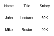
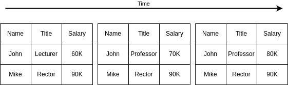
Example 6.1. A case study: imagine we have a database for managing personel, with the relation Employee(Name, Salary, Title, BirthDate). It is easy to know the salary of the employee, or its birthdate:
But it is often the case that we don’t only want to store the current state of things, but also a history. For instance, it can be interesting to store the employment history by extending the relation Employee(Name, Salary, Title, BirthDate, FromDate, ToDate). A dataset sample for this could be the following:
| Name | Salary | Title | BirthDate | FromDate | ToDate |
| John | 60K | Assistant | 9/9/60 | 1/1/95 | 1/6/95 |
| John | 70K | Assistant | 9/9/60 | 1/6/95 | 1/10/95 |
| John | 70K | Lecturer | 9/9/60 | 1/10/95 | 1/2/96 |
| John | 70K | Professor | 9/9/60 | 1/2/96 | 1/1/97 |
For the underlying system, the date columns FromDate and ToDate are no different from the BirthDate column, but it is obvious for us that the meaning is different: FromDate and ToDate need to be understood together as a period of time.
Now, to know the employee’s current salary, the query gets more complex:
Another interesting query that we can think of now is determining the salary history, i.e., all different salaries earned by the employee and in which period of time the employee was earning that salary. For our example, the result would be:
| Name | Salary | FromDate | ToDate |
| John | 60K | 1/1/95 | 1/6/95 |
| John | 70K | 1/6/95 | 1/1/97 |
But how can we achieve this?
One possibility is to print all the history, and let the user merge the pertinent periods.
Another one is to use SQL as a means to perform this operation: we have to find those intervals that overlap or are adjacent and that should be merged.
One way to do this in SQL is performing a loop that merges them in pairs, until there is nothing else to merge:
This loop is executed logN times in the worst case, where N is the number of tuples in a chain of overlapping tuples. After the loop, we have to deleted extraneous, non-maximal intervals:
The same thing can be achieved by unifying everything using a single SQL expression as
This is a complex query, and the logic is that if we want to merge the periods, we want to get a From and a To such that every period contained between From and To touches or intersect another period, and no period from outside From and To touches or interesects any of the periods inside:
 such that such that | ∀x :   ∃y : ∃y :  | ||
| ∧ | |||
∄x :  ∨ ∨ |
Now, the ∀ cannot be used in SQL, but we can use the fact that ∀x : P ≡¬¬
≡¬¬ ≡¬
≡¬ ≡ ∄x : ¬P
 ,
noting also that ¬
,
noting also that ¬ ≡ A∧¬B, and that is the query that we have shown above. An intuitive visualization is
the diagram in Figure 1.
≡ A∧¬B, and that is the query that we have shown above. An intuitive visualization is
the diagram in Figure 1.
Another possibility to achieve this temporal features is to make the attributes salary and title temporal, instead of the whole table. For this, we can split the information of the table into three tables:
Employee(Name, BirthDate)
EmployeeSal(Name, Salary, FromDate, ToDate)
EmployeeTitle(Name, Title, FromDate, ToDate)
Now, getting the salary history is easier, because we only need to query the table EmployeeSal:
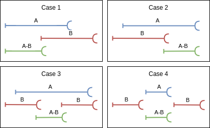
But, what if we want to obtain the history of the combinations of  ? We have to perform a temporal
join. Say we have the following tables:
? We have to perform a temporal
join. Say we have the following tables:
| Name | Salary | FromDate | ToDate |
| John | 60K | 1/1/95 | 1/6/95 |
| John | 70K | 1/6/95 | 1/1/97 |
| Name | Title | FromDate | ToDate |
| John | Assistant | 1/1/95 | 1/10/95 |
| John | Lecturer | 1/10/95 | 1/2/96 |
| John | Professor | 1/2/96 | 1/1/97 |
In this case, the answer to our temporal join would be:
| Name | Salary | Title | FromDate | ToDate |
| John | 60K | Assistant | 1/1/95 | 1/6/95 |
| John | 70K | Assistant | 1/6/95 | 1/10/95 |
| John | 70K | Lecturer | 1/10/95 | 1/2/96 |
| John | 70K | Professor | 1/2/96 | 1/1/97 |
For these, again, we could print the two tables and let the user make the suitable combinations, but it feels better to solve the problem using SQL. The query can be done as:
The four cases are depicted in Figure 2.
If we are using a system with embedded temporal capabilities, i.e., implementing TSQL2 (temporal SQL), we can let the system do it and just perform a join as we do it usually:
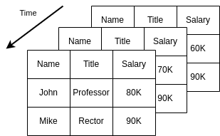
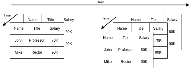
Time can be modelled in several ways, depending on the use case:
Linear: there is a total order in the instants.
Hypothetical: the time is linear to the past, but from the current moment on, there several possible timelines.
Directed Acyclic Graph (DAG): hypothetical approach in which some possible futures can merge.
Periodic/cyclic time: such as weeks, months... useful for recurrent processes.
We are going to assume a linear time structure.
Regarding the limits of the timeline, we can classify it:
Unbounded: it is infinite to the past and to the future.
Time origin exists: it is bounded on the left, and infinite to the future.
Bounded time: it is bounded on both ends.
Also, the bounds can be unspecified or specified.
We also need to consider the density of the time measures (i.e. what is an instant?). In this sense, we can classify the timeline as:
Discrete: the timeline is isomorphic to the integers. This means it is composed of a sequence of non-descomposable time periods, of some fixed minimal duration, named chronons and between a pair of chronons there is a finite number of chronons.
Dense: in this case, it is isomorphic to the ration numbers, with an infinite number of instants between each pair of chronons.
Continuous: the timeline is isomorphic to the real numbers, and again there is an infinite amount of instants between each pair of chronons.
Usually, a distance between chronons can be defined.
TSQL2 uses a linear time structure, bounded on both ends. The timeline is composed of chronons, which is the smallest possible granularity. Consecutive chronons can be grouped together into granules, giving multiple granularities and enable to convert from one another. The density is not defined and it is not possible to make questions in different granularities. The implementation is basically as discrete and the distance between two chronons is the amount of chronons in-between.
Temporal Types
Instant: a chronon in the time line.
Event: an instantaneous fact, something ocurring at an instant.
Event ocurrence time: valid-time instant at which the event occurs in the real world.
Instant set
Time period: the time between two instants (sometimes called interval, but this conflicts with the SQL type INTERVAL)
Time interval: a directed duration of time
Duration: an amount of time with a known length, but no specific starting or ending instants.
Positive interval: forward motion time.
Negative interval: backward motion time.
Temporal element: finite union of periods.
This way, in SQL92 we have the following Temporal Types:
DATE (YYYY-MM-DD)
TIME (HH:MM:SS)
DATETIME (YYYY-MM-DD HH:MM:SS)
INTERVAL (no default granularity)
And in TSQL2 we have:
PERIOD: DATETIME - DATETIME
The valid time of a fact is the time in which the fact is true in the modelled reality, which is independant of its recording in the database and can be past, present or future.
The transaction time of a fact is when the fact is current in the database and may be retrieved.
These two dimensions are orthogonal.
There are four types of tables:
Snapshot: these are usual SQL table, in which there is no temporality involved. What there is in the table is the current truth. They can be modified through time, but we only have access to the current truth.
Transaction Time: these tables are a set of snapshots tables, in which the past states can be queried for information, but they cannot be modified. When the current truth is modified, a snapshot is taken to preserved the history of changes.
Valid time: these are like transaction tables, but in which modification is permitted everywhere.
Bitemporal: in this case, we have valid time tables that can be taken snapshots to preserve full states.
Conceptual modeling is important because it focuses on the application, rather than the implementation. Thus, it is technology independent, which enhances the portability and the durability of the solution. It is also user oriented and uses a formal, unambiguous specification, allowing for visual interfaces and teh exchange and integration of information.
Semantically powerful data structures.
Simple data model, with few clean concepts and standard well-known semantics.
No aritifical time objects.
Time orthogonal to data structures.
Various granularities.
Clean, visual notations.
Intuitive icons/symbols.
Explicit temporal relationships and integrity constraints.
Support of valid time and transaction time.
Past to future.
Co-existence of temporal and tradicional data.
Query languages.
Complete and precise definition of the model.
In Figure 3, we can see three different ways to model a schema. Note how they are different, because the temporal attributes are dealt with differently in each of the models.
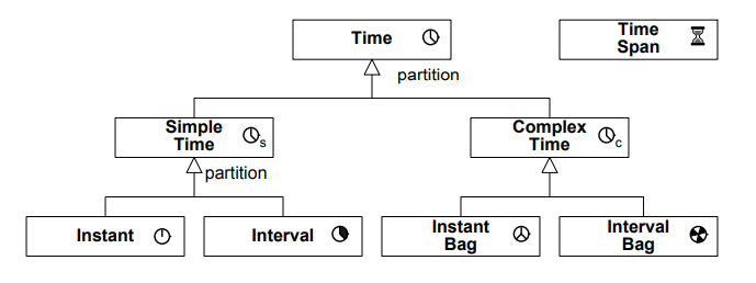
Time, SimpleTime and ComplexTime are abstract classes.
A temporal object is marked with the symbol  , and it indicates that the object has a set of periods of validity
associated.
, and it indicates that the object has a set of periods of validity
associated.
For example, if we have the relation Employee(name, birthDate, address, salary, projects (1..n)),
then, an instance of the relation can be:
|
Peter |
8/9/64 |
Rue de la Paix |
5000 |
{MADS, HELIOS} | [7/94-6/96] [7/97-6/98] Active |
| [7/96-7/97] Suspended | |||||
The red colored text are the life cycle information of the record.
The life cycle of an object can be continuous if there are no gaps between its creation and its deletion, or discontinuous if such gaps exist.
Non-temporal objects can be modeled with the absence of a lifecycle, or with a default life cycle which encodes that it is
always active. A usual option is to put it as ![[0,∞ ]](summary71x.png) .
.
The TSQL2 policy is that temporal operators are not allowed on non-temporal relations. So if we need to perform some kind of temporal operation in non-temporal relations, such as a join with a temporal relation, then we need to use the default life cycle.
A temporal attribute is marked with the symbol , and it indicates that the attribute itself has a lifecycle
associated.
For example, if we have the relation Employee(name, birthDate, address, salary, projects (1..n)),
then, an instance of the relation can be:
|
Peter |
8/9/64 |
Rue de la Paix | 4000 | [7/94-6/96] |
{MADS, HELIOS} |
| 5000 | [6/96-Now] | ||||
It is also possible to have temporal complex attributes, meaning attributes with subattributes. The temporality can be in either the full attribute, in which case a lifecyle will be attached to the whole attribute, or to a subattribute, in which case the lifecycle will be attached to only the subattribute.
For example, can have the relation Laboratory(name, projects (1..n) {name, manager, budget}) and
the relation Laboratory(name, projects (1..n) {name, manager , budget}).
An example of the first relation is:
| LBD
| |
| {(MADS,Chris,1500)} | [1/1/95-31/12/95] |
| {(MADS,Chris,1500),(Helios,Martin,2000)} | [31/12/95-Now] |
An example of the second relation is:
| LBD | ||||||||||||||||||
{(MADS,
|
||||||||||||||||||
In this second case, if we update manager, we add one new element to the manager history. If we update the project name, we would simply change it, because project is not temporal.
Attribute types / timestamping: none, irregular, regular, instants, durations,...
Cardinalities: snapshot and DBlifespan.
Identifiers: snapshot or DBlifespan.
MADS has no implicit constraint, even if they make sense, such as:
The validity period of an attribute must be within the lifecycle of the object it belongs to.
The validity period of a complex attribute is the union of the validity periods of its components.
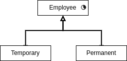
The life cycles are inherited from parent classes, and more temporal attributes can be added. For example:
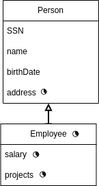
In this case, Employee is temporal, even though its parent is not. Employee inherits the temporal attribute address.
Another example:
In this case, both Temporary and Permanent are temporal objects.
In the case in which the child is also declared as temporal, it is called dynamic temporal generalization and in that case the objects maintains two lifecycles: the one inherited from its parent, and the one defined on itself. For example:
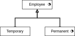
In this case, Permanent employees have two lifecycles: their lifecycle as a permanent and the inherited lifecycle as an employee. The redefined life cycle has to be including the one inherited.
A temporal relationship is also marked with the symbol , meaning that the relation between the objects possesses a
lifecycle.
Some usual constraints used in temporal relationships:
The validity period of a relationship must be within the intersection of the life cycles of the objects it links.
A temporal relationship can only link temporal objects.
Again, MADS does not impose any constraints.
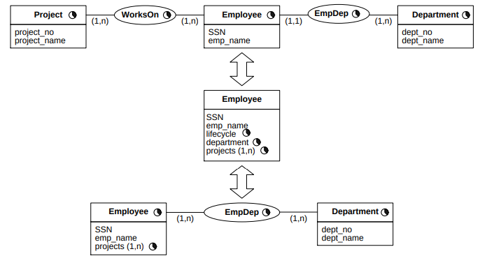
Example 8.2. Let’s see some temporal relationships.
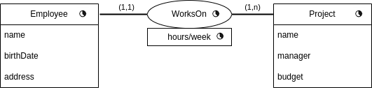
In this case, a possible data can be:
| Employee | |||||||||||||||||
e1
|
|||||||||||||||||
e2
|
|||||||||||||||||
| WorksOn | ||||||||||||||||||
w1
|
||||||||||||||||||
w2
|
||||||||||||||||||
w2
|
||||||||||||||||||
| Project | |||||||||||||||||
p1
|
|||||||||||||||||
p2
|
|||||||||||||||||
Another example, which is slightly different is the following:

In this case, the data can be:
| Employee | |||||||||||||||||
e1
|
|||||||||||||||||
e2
|
|||||||||||||||||
| WorksOn | |||||||||||||||
w1
|
|||||||||||||||
w2
|
|||||||||||||||
w2
|
|||||||||||||||
| Project | |||||||||||||||||
p1
|
|||||||||||||||||
p2
|
|||||||||||||||||
Now, only currently valid tuples are kept in the relationship. But for these, the history of hours/week is maintained.
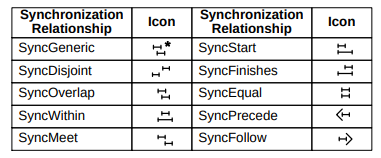
They describe temporal constraints between the life cycles of two objects and they are expressed with Allen’s operator extended for temporal elements:
before : interval i1 ends before i2 starts.
meets : interval i1 ends just when i2 starts.
overlaps : intervals i1 and i2 overlaps at some point.
during : interval i1 is contained inside interval i2.
starts : intervals i1 and i2 start at the same time.
finishes : intervals i1 and i2 finish at the same time.
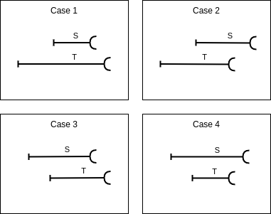
They can be visually seen in Figure
These relationships express a temporal constraint between the whole life cycles or the active periods.
Data type for periods is not available in SQL-92. Thus, a period is simulated with two Date columns: fromDate and toDate, indicating the beginning and end of the period, respectively. Some notes:
The special date ’3000-01-01’ denotes currently valid.
The periods are considered closed-open, [).
A table can be viewes as a compact representation of a sequence of snapshot tables, each one valid on a particular day.
Temporal statement apply to queries, modifications, views and integrity constraints. They are:
Current: applies to the current point in time. Example: what is Bob’s current position?
Time-sliced: applies to some point in time in the past or in the future. Example: what was Bob’s position on 1-1-2007?
Sequenced: applies to each point in time. Example: what is Bob’s position history?
Non-sequenced: applies to all points in time, ignoring the time-varying nature of tables. Example: when did Bob changed history?
Imagine we have the relation Incumbents(SSN,PCN,FromDate,ToDate) and we want to enforce that each employee has only one position at a point in time. If we use the key of the corresponding non-temporal table, (SSN,PCN), then we would not be able to enter the same employee for different periods. Thus, we need to somehow include the dates in the key. The options are: (SSN,PCN,FromDate), (SSN,PCN,ToDate) or (SSN,PCN,FromDate,ToDate). None of them captures the constraint that we want to enforce, because there are overlapping periods associated with the same SSN: we need a sequenced constraint, applied at each point in time. All constraints specified on a snapshot table have sequenced counterparts, specified on the analogous valid-time table.
Example 9.1. Employees have only one position at a point in time.
We have to decide how to timestamp current data. One alternative is to put NULL in the ToDate, which allows to identify current records by checking: WHERE ToDate IS NULL. But it possesses some disadvantages:
Users get confused with a data of NULL.
In SQL many comparisons with a NULL return false, so we might exclude some rows that should not be excluded from the query.
Other uses or NULL are not available.
Another approach is to set the ToDate to the largest value in the timestamp domain: ’3000-01-01’. The disadvantages of this are:
The DB states that something will be true in the far future.
’Now’ and ’Forever’ are represented in the same way.
There are different kind of duplicates in temporal databases:
Value equivalent: the values of the nontimestamp columns are equivalent. Example: all rows in Table 6.
Sequenced duplicates: when in some instant, the rows are duplicate. Example: rows 1 and 2 in the table.
Current duplicates: they are sequenced duplicates at the current instant. Example: rows 4 and 5 in the table.
Nonsequenced duplicates: the values of all columns are identical. Example: rows 2 and 3 in the table.
| SSN | PCN | FromDate | ToDate |
| 111223333 | 120033 | 1996-01-01 | 1996-06-01 |
| 111223333 | 120033 | 1996-06-01 | 1996-10-01 |
| 111223333 | 120033 | 1996-06-01 | 1996-10-01 |
| 111223333 | 120033 | 1996-10-01 | Now |
| 111223333 | 120033 | 1997-12-01 | Now |
To prevent value equivalent rows: we define a secondary key using UNIQUE(SSN,PCN).
To prevent nonsequenced duplicates: UNIQUE(SSN,PCN,FromDate,ToDate).
To prevent current duplicates: no employee can have two identical positions at the current time:
To prevent current duplicates, assuming no future data, we notice that current data will have the same ToDate, so we set UNIQUE(SSN,PCN,ToDate).
To prevent sequenced duplicates, we do as with the trigger for sequenced primary keys, but disregarding NULL values (because now we are not making a key UNIQUE+NOTNULL, but only UNIQUE):
To prevent sequenced duplicates, asumming only modifications to current data, we can use UNIQUE(SSN, PCN, ToDate).
Now, we want to enforce that each employee has at most one position. In a snapshot table, this would be equivalent to UNIQUE(SSN), and now the sequenced constraint is: at any time each employee has at most one position, i.e., SSN is sequenced unique:
We can also think about the nonsequenced constraint: an employee cannot have more than one position over two identical periods, i.e. SSN is nonsequenced unique: UNIQUE(SSN,FromDate,ToDate).
Or current constraint: an employee has at most one position now, i.e. SSN is current unique:
We want to enforce that Incumbents.PCN is a foreign key for Position.PCN. There several possible cases, depending on what tables are temporal.
In this case, if we want the PCN to be a current foreign key, the PCN of all current incumbents must be listed in the current positions:
Or it can be a sequenced foreign key:
A contiguous history is such that there are no gaps in the history. Enforcing contiguous history is a nonsequenced constraint, because it requires examining the table at multiple points of time.
We can also have the situation that Incumbents.PCN is a FK for Position.PCN and Position.PCN defines a contiguous history. In this case, we can omit the part of searching for the P2 that extends a P that ends in the middle of I.
Current FK:
We have the relations:
| SSN | FirstName | LastName | BirthDate |
| SSN | PCN | FromDate | ToDate |
| SSN | Amount | FromDate | ToDate |
| Position
| |
| PCN | JobTitle |
Say we want to obtain Bob’s current position. Then:
And Bob’s current position and salary? Current joins:
And if we want to get what employees have currently no position?
A timeslice query extracts a state at a particular point in time. They require an additional predicate for each temporal tables: they are basically the same as checking the current state, but with a different date.
For example: Bob’s position at the beginning of 1997?
A sequenced query is such that its result is a valid-time table. They use sequenced variants of basic operations:
Sequenced selection: no change:
Sequenced projection: include the timestamp columns in the select list, because if not we would obtain several values for the same employees:
If we want to remove the duplicates here, we need to coalesce the results.
Sequenced sort: in this case we require the result to be ordered at each point in time. This can be accomplished by appending the start and end time columns in the ORDEER BY:
It can also be done by omitting the timestamp columns.
Sequenced union: a UNION ALL (retaining duplicates) over temporal tables is automatically sequenced if the timestamp columns are kept:
Sequenced join: imagine we want to determine the salary and position history for each employee. This implies a sequenced join between Salary and Incumbents. It is supposed that there are no duplicate rows in the tables: at each point in time an employee has one salary and one position. In SQL, a sequenced join requires four select statements and complex inequality predicates and the following code does not generate duplicates. This is why UNION ALL is used without problems, and being more efficient than UNION, which does a lot of work for removing non-ocurring duplicates5 .
This can also be done using CASE, which allows to write the query in a single statement: the first case simulates a maxDate function of the two arguments, the second one a minDate function. The condition in the WHERE ensures that the period of validity is well formed:
Another way to do the sequenced join is using functions:
Temporal difference: the usual difference is implemented in SQL with EXCEPT, NOT EXISTS or NOT IN. For example, if we want to list the employees who are department heads (PCN=1234) but are not also professors (PCN=5555), we can do it as:
But the sequenced difference is a bit more complex. There are four possible cases, depicted in Figure 6.
The SQL query is:
Nonsequenced operators are straightforward: they ignore the time-varying nature of the tables.
Example 9.2. List all the salaries, past and present, of employees who had been lecturer at some time:
When did employees receive raises?
Remove nonsequenced duplicates from Incumbents:
Remove value-equivalent rows from Incumbents:
Remove current duplicates from Incumbents:
Say we have two relations:
| SSN | DNumber | FromDate | ToDate |
| SSN | Amount | FromDate | ToDate |
And we want the maximum salary. The non-temporal version is straighforward:
And the maximum salary by department:
But the temporal version is not that easy. We have to do as in this visual example:
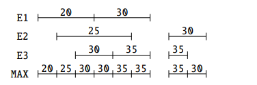
The steps to follow are:
Compute the periods on which a maximum must be calculated.
Compute the maximum for the periods.
Coalesce the results (as we have already seen)
Now, we want to compute the history of maximum salary by deparment:
Compute by department the periods on which a maximum must be calculated.
Compute the maximum salary for these periods.
Coalesce the results.
Now we have the tables:
| SSN | DNumber | FromDate | ToDate |
| PNumber | DNumber | FromDate | ToDate |
| SSN | PNumber | FromDate | ToDate |
And say we want to get the employees that are working all projects of the department to which they are affiliated.
Nontemporal version:
Sequenced division: Case1. Only WorksOn is temporal.
Construct the periods on which the division must be computed.
Compute the division.
Coalesce.
Sequenced division: Case 2. Only Controls and WorksOn are temporal. In this case, employees may work on projects controlled by departments different from the department to which they are affiliated.
Construct the periods on which the division must be computed.
Compute the division of these periods.
Coalesce.
Sequenced division: Case 3. Only Affiliation and WorksOn are temporal. Again, employees may work in projects controlled by departments different from the department to which they are affiliated.
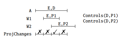
The steps are conceptually the same, so let’s go with SQL:
Sequenced division, Case 4. The three tables are temporal.
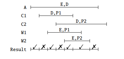
Oracle 9i included support for transaction time. Flashback queries allow the application to access prior transaction-time states of their database: they are transaction timeslice queries. Database modifications and conventional queries are temporally upward compatible.
Oracle 10g extended flashback queries to retrieve all the versions of a row between two transaction times. It also allowed tables and databases to be rolled back to a previous transaction time, discarding changes after that time.
Oracle 10g Workspace Manager includes the period data type, valid-time support, transaction-time support, bitemporal support and support for sequenced primary keys, sequenced uniqueness, sequenced referential integrity and sequenced selection and projection.
Oracle 11g does not rely on transient storage like the undo segments, it records changes in the Flashback Recovery Area. Valid-time queries were also enhanced.
Teradata Database 13.10 introduced the period data type, valid-time support, transaction-time support, timeslices, temporal upward compatibility, sequenced primary key and temporal referential integrity constraints, nonsequenced queries, and sequenced projection and selection.
Teradata Database 14 adds capabilities to create a global picture of an organization’s business at any point in time.
IBM DB2 10 includes the period data type, valid-time support (termed business time), transaction-time support (termed system time), timeslices, temporal upward compatibility, sequenced primary keys, and sequenced projection and selection.
SQL2011 has temporal support:
Application-time period tables: valid-time tables. They have sequenced primary and foreign keys, support single-table valid-time sequenced insertions, deletions and updates, and nonsequenced valid-time queries.
They contain a PERIOD clause with an user-defined period name. Currently restricted to temporal periods only. They must contain two additional columns, to store the start time and the end time of a period associated with the row, whose values are set by the user. The user can also specify primary key/unique constraints to ensure that no two rows with the same key value have overlapping periods, as well as referential integrity constraints to ensure that the period of every child row is completely contained in the period of exactly one parent row or in the combined period of two or more consecutive parent rows.
Queries, inserts, updates and deletes behave exactly like in regular tables. Additional syntax is provided on UPDATE and DELETE statements for partial period updates and deletes.
We can create an application-time period table as
The PERIOD clause automatically enforces the constraint end_date > start_date. The name of the period can be any user-defined name. The period is closed-open, [).
To insert a row into an application-time period table, the user needs to provide the start and end time of the period for each row. The time values can be either in the past, current or future.
All rows canbe potentially updated. Users are allowed to update the start and end columns of the period associated with each row and when a row is updated using the regular UPDATE statement, the regular semantics apply. Additional syntax is provided for UPDATE statements to specify the time period during which the update applies, and only rows that lie within the specified period are impacted in that case. This can lead to row splits, if the modification lies in the middle of the period of the row. Users are not allowed to update the start and end columns of the period associated with each row under this option.
Also, all rows can be potentially deleted. Again, normal semantics apply unless we use the syntax provided to specify the time period during which the delete applies, so only rows lying inside the indicated period are impacted. This can also lead to row splits.
To query a table, normal syntax applies. If we want to retrieve the current department of John:
Or if we want the number of different departments in which John worked since Jan 1 96:
Benefits of application-time period tables:
Most business data is time sensitive.
DB systems today offer no support for associating user-maintained time periods with rows nor enforcing constraints such as ’an employee can be in only one department in any given period’.
Updating/deleting a row for a part of its validity period.
Currently, applications take the responsibility for managing such requirements.
The major issues are the complexity of the code and its poor performance.
These table provide:
Significant simplification of application code
Significant improvement in performance
Transparent to legacy applications
System-versioned tables: transaction-time tables. They have transaction-time current primary and foreign keys, support transaction-time current insertions, deletions and updates, and transaction-time current and nonsequenced queries.
These tables contain a PERIOD clause with a pre-defined period name (SYSTEM_TIME) and specify WITH SYSTEM VERSIONING. They must contain two additional columns, to store the start time and the end time of the SYSTEM_TIME period, whose values are set by the system, not the user. Unlike regular tables, system-versioned tables preserve the old versions of rows as the table is updated.
Rows whose periods intersect the current time are called current system rows, all others are called historical system rows. Only current system rows can be updated or deleted and the constraints are enforced only on current system rows.
To create a table:
The PERIOD clause automatically enforces the constraint system_end > system_start and the name of the period must be SYSTEM_TIME. The period is closed, open [).
When a row is inserted into a system-versiones table, the SQL-implementation sets the start time to the transaction time and the end time to the largest timestamp value. All rows inserted in a transaction will get the same values for the start and end columns.
When a row is updated the SQL-implementation insert the ’old’ version of the row into the table before updating the row, setting its end time and the start time of the updated row to the transaction time. Users are not allowed to modify the start nor end time.
When a row is deleted, the SQL-implementation does not actually delete the row, but sets its end time to the transaction time.
To query a system-versiones table, existing syntax for querying regular tables is applicable. Additional syntax is provided for expressing queries involving system-versioned tables in a more succint manner:
If none of this clause are specified, the system queries only current system tables.
Benefits of system-versioned tables:
Today’s DB systems focus mainly on managing current data, providing almnost no support for managing historical data, while some applications have an inherent need for preserving old data. Also, regulatory and compliance laws require keeping old data around for a certain period of time. Currently, applications take on this responsibility.
The major issues are as before: complexity of the code and poor performance.
System-versioned tables provide:
Significant simplification of application code.
Significant improvement in performance.
Transparent to legacy applications.
System-versiones application-time period tables: bitemporal tables. They support temporal queries and modifications of combinations of the valid-time and transaction-time variants. These tables support features of both application-time period tables and system-versioned tables.
To create a table:
Say we want to make the following update: On 15/12/97, John is loaned to department M12 starting from 01/01/98 to 01/07/98:
Or in 15/12/98, John is approved for a leave of absence from 1/1/99 to 1/1/2000:
A spatial database is a database that needs to store and query spatial objects, such as points (a house in a city), lines (a road) or polygons (a country). Thus, a spatial DBMS is a DBMS that manages data existing in some space:
2D or 2.5D: integrated circuits (VLSI design) or geographic space (GIS, urban planning).
2.5D: elevation.
3D: medicine (brain models), biological research (moledule structures), architecture (CAD) or ground models (geology).
The supporting technology needs to be able to manage large collections of geometric objects, and major commercial and open source DBMSs provide spatial support.
Spatial databases are important because queries to databases are posed in high level declarative manner, usually with SQL, which is popular in the commercial DB world. Also, although the standard SQL operates on relatively simple data types, additional spatial data types and operations can be defined in spatial databases.
A geographic information system (GIS) is a system designed to capture, store, manipulate, analyze, manage and present geographically-referenced data, as well as non spatial data. It can be used to establish connections between different elements using geography operations, such as the location, the proximity or the spatial distribution. There are plenty of commercial and open source systems of this kind, but with limited temporal support.
A GIS can be seen as a set of subsystems:
Data processing: data acquisition, input and store.
Data analysis: retrieval and analysis.
Information use: it is needed an interaction between GIS group and users to plan analytical procedures and data structures. The users of GIS are researches, planners or managers.
Management system: it has an organizational role, being a separate unit in a resource management. An agency offering spatial DB and analysis services.
There are many fields involved in the development of GIS: geography, cartography, remote sensing, photogrammetry, geodesy, statistics, operations research, mathematics, civil engineering and computer science, with computer aided design (CAD), computer graphics, AI and DBMS.
There are several possible architectures for a GIS:
Ad Hoc Systems: they are developed for a specific problem. They are not modular, nor reusable nor extensible, nor friendly but are very efficient.
Loosely coupled approach: structured information and geometry are stored at different places:
There is a RDBMS for non spatial data.
There is a specific module for spatial data management.
This allows for modularity, but there are two heterogeneous models in use. This makes it more difficult to model, integrate and use. Also, there is a partial loss of basic DBMS functionality (concurrency, optimization, recovery, querying).
Integrated approach: this approach is an extended relational system, which makes it modular, extensible, reusable and friendly.
Going from 3D to 2D for Earth representation always involves a projection, so information on the projection is essential for applications analyzing spatial relationships and the choice of the projection used can influence the results. Also, the Earth is a complex surface whose shape and dimensions cannot be described with mathematical formulas. Two main reference surfaces are used to approximate the shape of the Earth: the ellipsoid and the geoid.
The geoid is a reference model for the physical surface of the Earth. It is defined as the equipotential surface of the Earth’s gravity field which best fits the global mean sea level and extended through the continents. It is used in geodesy but it is not very practical to produce maps. Also, since its mathematical description is unknown, it is impossible to identify mathematical relationships for moving from the Earth to a map.
An ellipsoid is a mathematically defined surface that approximates the geoid. It is the 3-dimensional version of an ellipse.
The flattening measures how much the symmetry axis is compressed relative to the equatorial radius, it is computed by

For the Earth, f ~ : the difference of the major and minor semi-axis is approximately 21 km. The ellopsoid is
thus used to measure locations, using the latitude and the longitude, for points of interest. These locations on the
ellipsoid are then projected onto a mapping plane. Note that different regions of the world use a different reference
ellipsoid that minimize the differences between the geoid and the ellipsoid. For Belgium, the ellipsoid is GRS80 or
WGS84, with a = 6378137 m and f =
: the difference of the major and minor semi-axis is approximately 21 km. The ellopsoid is
thus used to measure locations, using the latitude and the longitude, for points of interest. These locations on the
ellipsoid are then projected onto a mapping plane. Note that different regions of the world use a different reference
ellipsoid that minimize the differences between the geoid and the ellipsoid. For Belgium, the ellipsoid is GRS80 or
WGS84, with a = 6378137 m and f =  .
.
This is done because the physical Earth has excursions of +8km and -11km, so the geoid’s total variation goes from -107m to +85m compared to a perfect ellipsoid.
Latitude and longitude are measures of the angles (in degrees) from the center of the Earth to a point on the Earth’s surface. The latitude measures angles in the North-South direction, with the equator being at 0º. The longitude measures angles in the East-West direction, with the prime meridian at 0º.
Note that they are not uniform units of distance, because the degrees change differently depending on where in the map we look at. Only along the equator the distance represented by one degree of longitude approximates the distance represented by one degree of latitude.
To produce a map, the curved surface of the Earth, approximated by an ellipsoid is transformed into the flat plane
of the map by means of a map projection. A point on the reference surface of the Earth with coordinates  is
transformed into Cartesian coordinates
is
transformed into Cartesian coordinates  representing the positions on the map plane. Each projection causes
deformations in one or another way.
representing the positions on the map plane. Each projection causes
deformations in one or another way.
Map projections can be categorized in four ways: shape used, angle, fit and properties.
Different shapes can be used for projection, commonly either a flat plane, a cylinder or a cone. Note that cylinders and cones are flat shapes, but they can be rolled flat without introducing additional distorsion.
According to this categorization, the projection can be:
Cylindrical: coordinates projected onto a cylinder. These work best for rectangular areas.
Conical: coordinates projected onto a cone. These work best for triangle shaped areas.
Azimuthal: coordinates projected directly onto a flat planar surface. These work best for circular areas.
The angle referes to the alignment of the projection surface, measured as the angle between the main axis of the Earth and the main symmetry axis of the projection surface:
Normal: the two axes are parallel.
Transverse: the two axes are perpendicular.
Oblique: the two axes are at some other angle.
Ideally the plane of projection is aligned as closely as possible with the main axis of the area to be mapped, minimizing distorsion and scale errors.
The fit is a measure of how closely the projection surface fits the surface of the Earth:
Tangent: the projection surface touches the surface of the Earth.
Secan: the projection surface slices through the Earth.
Distorsion occurs whenever the projection surface is not touching or intersecting the surface of the Earth. Secant projections usually reduce scale errors, because the two surface intersect in more places and the overall fits tends to be better. A globe is the only way to represent the entire Earth without significant scale errors.
With different projections, different measures are preseved:
Conformal: preserve shapes and angles. Recommended for navigational charts and topographic maps.
Equal area: preserve areas in correct relative size. Best suited for thematic mapping.
Equidistant: preserve distance (only possible at certain locations or in certain directions). Best suited when measuring distance from a point.
True-direction: preserve accurate directions.
It is impossible to construct a map that is equal-area and conformal.
The data modeling of spatial features requires for multiple views of space (discrete and continuous; 2D, 2.5D and 3D), multiple representation of the data, at different scales and from different viewpoints, several spatial abstract data types (point, line, area, set of points,...) and explicit spatial relationships (crossing, adjacency,...).
Let’s see this requirements in depth. First, we have interaction requirements:
Visual interactions: map displays, information visualizations and graphical queries on maps.
Flexible, context-dependent interactions.
Multiple user profiles (a highway can have constructors, car drivers, hikers,...)
Multiple instantiations (a building may be a school and a church).
Practical requirements:
Huge dataset: collecting new data is expensive, so reusing highly heterogeneous datasets is a must... but it is very complex. The integration requires understanding, so a conceptual model is important.
Integration of DB with different space/time granularity.
Coexistence with non-spatial and non-temporal data.
Reengineering of legacy applications.
Interoperability.
Thus, conceptual modelling is important because it focuses on the application, it is technology independent, which increases portability and durability. It is user oriented and uses a formal unambiguous specification, with the support of visual interfaces for data definition and manipulation. It is the best vehicle for information exchange and integration.
It has a good expressive power, with a simple data model, with few clean concepts and standard, well-known semantics. There are no artificial constructs and space, time and data structures are treated as orthogonal. It provieds a clean, visual notation and intuitive icons and symbols, providing a formal definition and an associated query language.
As with temporal DB, in spatial DB there are multiple ways to model the reality, each with its own characteristics. For example:
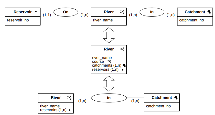
And there is also a MADS Spatial Type Hierarchy:
We need to keep in mind that the types are topologically closed: all geometries include their boundary.
Geo, SimpleGeo and ComplexGeo are abstract classes.
Point: its boundary is the empty set.
Line: it can be of several types:
Its boundary is composed of the extreme points, if any.
Surface: it is define by 1 exterior boundary and 0 or more interior boundaries, defining its holes:
The following are not surfaces:
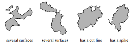
Complex geometries: a complex geometry is a geometry composed of several sub-geometries. Its boundary is defined recursively as the spatial union of:
The boundaries of its components that do not intersect with other components.
The intersecting boundaries that do not lie in the interior of their union.
If we have two geometries, a and b, then
![B (a∪ b) = [B (a)- b]∪[B (b) - a]∪ [(B (a)∩ b)∪ (B (b)∩ a)- I(a∪ b)],](summary83x.png)
where B is the boundary of x and I
 is the interior of x. A sample classification of different cases is the
following:
is the interior of x. A sample classification of different cases is the
following:
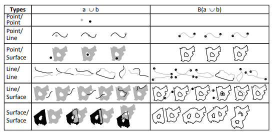
A topological predicate specifies how two geometries relate to each other. It is based on the definition of their boundary
B , interior I
 , and exterior E
 , and their dimension Dim
 , which can be -1,0,1 or 2 (-1 is for the empty set).
The dimensionally extended 9-intersection matrix (DE-9IM) is a matrix used for defining predicates. It is based
in the following template:
, which can be -1,0,1 or 2 (-1 is for the empty set).
The dimensionally extended 9-intersection matrix (DE-9IM) is a matrix used for defining predicates. It is based
in the following template:
| Interior | Boundary | Exterior | |
| Interior | Dim | Dim | Dim |
| Boundary | Dim | Dim | Dim |
| Exterior | Dim | Dim | Dim |
It is coded using a dense notation with a string of 9 characters, to represent the cells of the matrix. The possible characters are:
T: non-empty intersection.
F: empty intersection.
0: intersection is a point.
1: intersection is a line.
2: intersection is a surface.
*: it is irrelevant.
Example 13.1. Disjoint is true if their intersection is empty. So, it is
![Disjoint (a,b) = [I(a)∩ I(b) = ∅]∧[I(a)∩ B (b) = ∅]∧ [B (a)∩ I(b) = ∅]∧ [B (a)∩ B (b) = ∅].](summary100x.png)
Then, it can be coded as ’FF*FF****’.
Let’s see some predicates:
Meets ⇐⇒
⇐⇒![[I(a)∩ I(b) = ∅]](summary102x.png) ∧
∧![[a ∩b ⁄= ∅]](summary103x.png) ∧
∧![[Dim (a ∩b) = 0]](summary104x.png) . Some geometries that satisfy
it:
. Some geometries that satisfy
it:
And some that don’t:
Adjacent ⇐⇒
⇐⇒![[I(a)∩ I(b) = ∅]](summary106x.png) ∧
∧![[a ∩ b ⁄= ∅]](summary107x.png) ∧
∧![[Dim (a ∩ b) = 1]](summary108x.png) . Some geometries that satisfy
it:
. Some geometries that satisfy
it:
And an example that doesn’t:

Touches ⇐⇒
⇐⇒![[I (a) ∩I (b) = ∅]](summary110x.png) ∧
∧![[a∩ b ⁄= ∅]](summary111x.png) ⇐⇒ Meets
⇐⇒ Meets ∨ Adjacent
 .
.
Crosses ⇐⇒
⇐⇒![[Dim (I(a)∩ I(b)) < max {Dim (I(a)),Dim (I (b))}]](summary115x.png) ∧
∧![[a ∩b ⁄= a]](summary116x.png) ∧
∧![[a∩ b ⁄= b]](summary117x.png) ∧
∧![[a∩ b ⁄= ∅]](summary118x.png) .
Some geometries that satisfy it:
.
Some geometries that satisfy it:
Overlaps ⇐⇒
⇐⇒![[Dim (I(a)) = Dim (I(b)) = Dim (I(a)∩ I(b))]](summary120x.png) ∧
∧![[a∩ b ⁄= a]](summary121x.png) ∧
∧![[a ∩ b ⁄= b]](summary122x.png) . Some geometries
that satisfy it:
. Some geometries
that satisfy it:
Contains ⇐⇒ Within
 ⇐⇒
⇐⇒![[I(a)∩ I(a) ⁄= ∅]](summary125x.png) ∧
∧![[a∩ b = b]](summary126x.png) . Some geometries that satisfy
it:
. Some geometries that satisfy
it:
Disjoint ⇐⇒ a ∩ b = ∅⇐⇒ Intersects
 .
.
Equals ⇐⇒
⇐⇒![[a ∩b = a]](summary130x.png) ∧
∧![[a ∩b = b]](summary131x.png) ⇐⇒
⇐⇒ ∪
∪ = ∅.
= ∅.
Covers ⇐⇒ a ∩ b = b ⇐⇒ b - a = ∅ (same as contains
 but it can have empty interior).
Encloses ⇐⇒ Surrounded
 : the definition is involved, depending of whether a is a (set of) line(s) or a
(set of) surface(s). Some examples that verify it:
: the definition is involved, depending of whether a is a (set of) line(s) or a
(set of) surface(s). Some examples that verify it:
Objects can be defined as spatial:
Country  |
| name |
| population |
Both non-spatial and spatial objects types can have spatial attributes. The domain of a spatial attribute is a spatial type, and can be multi-values. A spatial attribute of a spatial object type may induce a toplogical constraint (e.g. the capital of a country is located within the geometry of the country), but is is not necessarilly the case: it depends on application semantics and the application schema must explicitly state these constraints.
| Client |
| name |
| address |
location |
| Country |
| name |
| population |
| capital |
rivers(1,n)  |
| Road |
| name |
| responsible |
| stations(1,n) |
Spatial attributes can be a component of a complex and/or multivalued attribute. It is usual to keep both thematic (alphanumeric) and location data for attributes, as a capital, for example. This allows to print both the name and the location in a map. However, in real maps the toponyms have also a location: there are precise cartographic rules for placing them, so it is a semi-automatic process.
| Country |
||||||
| name | ||||||
| population | ||||||
capital
|
||||||
provinces(1,n)
|
||||||
Representing a concept as a spatial object or as a spatial attribute depends on the application and it is determined by the relative importance of the concept. This has implications in the way of accessing the instances of the concept. For example, buildings:
As spatial objects: the application can access a building one by one.
As spatial attributes: the access to a building must be made through the land plot containing it.
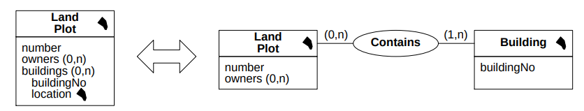
Spaciality is inherited through generalization, based on the well-known substitutability principle in OOP. For simple inheritance it is not necessary to re-state the geometry in the subtype and, as usual, spatiality can be added to a subtype, so that only instances of the subtype have associated spaciality.
This arises when a spaciality is re-stated in a subtype:
Refinement: it restricts the inherited property. The value remains the same in the supertype and the subtype.
Redefinition: it keeps substitutability with respect to typing and allows dynamic binding.
Overloading: relaxes substitutability, inhibiting dynamic binding.
Spatiality is inherited from several supertypes, and this creates an ambiguity when referring to the spatiality of the subtype. Several policies have been proposed for solving this issue in the OO community, and the most general policy is: all inherited properties are available in the subtype, is the user who must disambiguate in queries.
Spatiality can also be defined for relationships, and it is orthogonal to the fact that linked object types are spatial. If a spatial relationship relates spatial types, spatial constraints may restrict the geometries.
They are specified on a relationship type that links at least two spatial types, and constraint the spatiality of the instances of the related types. Many topological constraints can be defined using the DE-9IM. The conceptual model depicts only the most general ones. These are:
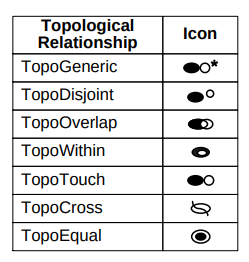
Traditional aggregation relatiomnships can link spatial types. Usually, aggregation has exclusive semantics, stated by cardinalities in the component role. Also, the spatiality of the aggregation is often partitioned into the spatiality of the components.
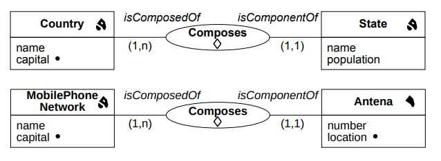
Note that it is not the case for the second example, where the spaciality of Antena corresponds to its coverage, so the same location can be covered by several antennas. Spaciality of the aggregation is the spatial union of the spaciality of the antennas.
They are also referred to as continuous fields, and allow to represent phenomena that change in space and/or time, such as elevation (to each point there is an associated real number), population (to each point there is an associated integer) or temperature (to each point in space there is an associated real number, which evolves over time). At the conceptual level, it can be represented as a continuous function, so operators for manipulating fields can be defined. At the logical level it can be implemented in several ways:
Raster: discretize the space into regular cells and assign a value to each cell.
TIN: keep values at particular locations and use interpolation for calculating the value at any point.
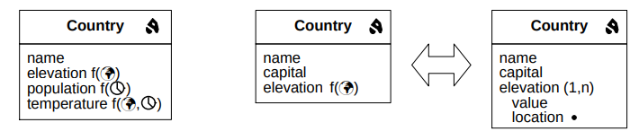
This model try to represent an infinite sets of points of the Euclidean space in a computer. There two alternative representations:
Object-based model (vector): describes the spatial extent of relevant objects with a set of points. It uses pints, lines and surfaces for describing spaciality and the choice of geometric types is arbitrary, varying across systems.
Field-based model (raster): each point in space is associated with one or several values, defined as continuous functions.
Tesselation is the decomposition of the plane into polygonal units, which might be regular or irregular, depending on whether the polygonal units are of equal size:
Regular tesselation is used for remote sensing data, while irregular tesselation is used for zoning in social, demographic or economic data. A spatial Object is represented by the smallest subset of pixels that contains it.
They provide a digital (finite) representation of an abstract model of space. DEMs are useful to represent a natural phenomenon that is a continuous function of the 2D space. They are based on a finite collection of sample values, and the rest are obtained by interpolation.
Triangulated irregular networks (TINs) are based on a triangular partition of the 2D space:
No assumption is made on the distribution and location of the vertices of the triangles and the elevation value is recorded at each vertex. The value for the rest of the points is interpolated using linear interpolation of the 3 vertices of the triangle that contains the point.
There are three comonly used rperesentations: spaghetti, network and topological, which mainly differ in the expression of topological relationships among the component objects.
The geometry of any object is described independently of the rest, so no topology is stored in the model: the topological relationships must be computed on demand. This implies representation redundancy, but enables heterogeneous representations mixing points, polylines and regions without restrictions.
Advantages:
Simplicity.
Provides the end user with easy input of new objects into the collection.
Drawbacks:
Lack of explicit information about topological relationships among spatial objects.
Redundancy: problem with large datasets and source of inconsistency.
It is destined for network or graph based applications. The topological relationships among points and polylines are stored:
Nodes: distinguished points that connect a list of arcs.
Arcs: polyline that starts at a node and ends at a node.
Nodes allow efficient line connectivity test and network computations. There are two types of points: regular points and nodes.
Depending on the implementation, the network is planar or nonplanar:
Planar network: each edge intersection is recorded as a node, even if it does not correspond to a real-world entity.
Nonplanar network: edges may cross without producing an intersection.
It is similar to the network model, except that the network is plannar. It induces a planar subdivision into adjacent polygons, some of which may not correspond to actual geographic objects:
Node: represented by a point and the list of arcs starting/ending at it. And isolated point (empty list of arcs) identifies the location of point features, such as towers, point of interest,...
Arc: features its ending points, list of vertices and two polygons having the arc as a common boundary.
Polygon: represented by a list of arcs, each arc being shared with a neighbor polygon.
Region: represented by one or more adjacent polygons.
There is no redundancy: each point/line is stored only once.
Advantages: efficient computation of topological queries, and up-to-date consistency.
Drawbacks: some DB objects have no semantics in real world, and the xomplexity of the structure may slow down some operations.
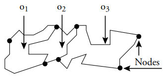
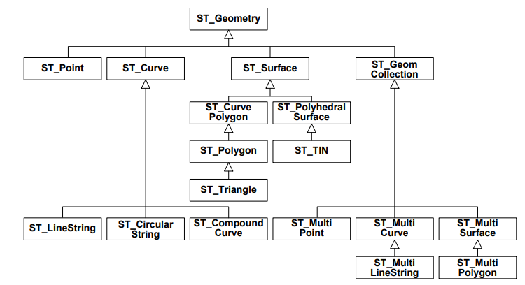
ST_Geometry, ST_Curve and ST_Surface are not instantiable types.
Represents 0D, 1D and 2D geometries that exist in 2D, 3D or 4D. Geometries in ℝ2 have points with  coordinate
values, in ℝ3 it is
coordinate
values, in ℝ3 it is  or
or  and in ℝ4 it is
  .
.
The z usually represents altitude.
The m usually represents a measurement: it is key to support linear networking applications, such as street routing, transportation or pipelining.
Geometry values are topolofically closed, i.e., they include their boundary.
All locations in a geometry are in the same spatial reference system (SRS), and geometric calculations are done in the SRS of the first geometry in the parameter list of a routine. The return value is also in the SRS of the first parameter.
ST_Dimension: returns the dimension of a geometry.
ST_CoordDim: returns the coordinate dimension of a geometry.
ST_GeometryType: returns the type of the geometry as a CHARACTER VARYING value.
ST_SRID: observes and mutates the spatial reference system identifier of a geometry.
ST_Transform: returns the geometry in the specified SRS.
ST_IsEmpty: tests if a geometry corresponds to the empty set.
ST_IsSimple: tests if a geometry has no anomalous geometric points.
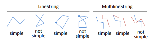
ST_IsValid: tests if a geometry is well formed.
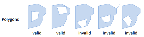
ST_Is3D: tests whether a geometry has z coordinate.
ST_IsMeasured: tests whether a geometry has m coordinate.
ST_Boundary: returns the boundary of a geometry.
ST_Envelope: returns the bounding rectangle of a geometry.
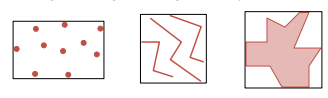
ST_ConvexHull: returns the convex hull of a geometry.
ST_Buffer: returns the geometry that represents all points whose distance from any point of a geometry is less than or equal to a specified value.
ST_Union: returns the geometry that represents the point set union of two geometries.
ST_Intersection: returns the geometry that represent the point set intersection of two geometries.
ST_Difference: returns the geometry that represents the point set difference of two geometries.
ST_SymDifference: returns the geometry that represents the point set symmetric difference of two geometries.
ST_Distance: returns the distance between two geometries.
ST_WTKToSQL: returns the geometry for the specified well-known text representation.
ST_AsText: returns the well-known text representation for the specified geometry.
ST_WKBToSQL: returns the geometry for the specified well-known binary representation.
ST_AsBinary: returns the well-known binary representation for the specified geometry.
ST_GMLToSQL: returns the geometry for the specified GML representation.
ST_AsGML: returns the GML representation for the specified geometry.
ST_GeomFromText: returns a geometry, which is transformed from a CHARACTER LARGE OBJECT value that represents its well-known text representation.
ST_GeomFromWKB: returns a geometry, which is transformed from a BINARY LARGE OBJECT value that represents its well-known binary representation.
ST_GeomFromGML: returns a geometry, which is transformed from a CHARACTER LARGE OBJECT value that represents its GML representation.
Boundary of a geometry: set of geometries of the next lower dimension.
ST_Point or ST_MultiPoint: empty set.
ST_Curve: start and end ST_Point values if nonclosed, empty set if closed.
ST_MultiCurve: ST_Point values that in the boundaries of an odd number of its element ST_Curve values.
ST_Polygon: its set of linear rings.
ST_Multipolygon: set of linear rings of its ST_Polygon values.
Arbitrary collection of geometries whose interiors are disjoint: geometries drawn from the boundaries of the element geometries by application of the mod 2 union rule.
The domain of geometries considered consists of those values that are topologically closed.
Interior of a geometry: points that are left when the boundary is removed.
Exterior of a geometry: points not in the interior or boundary.
ST_Equals: tests if a geometry is spatially equal to another geometry.
ST_Disjoint: tests if a geometry is spatially disjoint from another geometry.
ST_Intersects: tests if a geometry spatially intersects another geometry.
ST_Touches: tests if a geometry spatially touches another geometry.
ST_Crosses: tests if a geometry spatially crosses another geometry.
ST_Within: tests if a geometry is spatially within another geometry.
ST_Contains: tests if a geometry spatially contains another geometry.
ST_Overlaps: tests if a geometry spatially overlaps another geometry.
ST_Relate: tests if a geometry is spatially related to another geometry by testing for intersections between their interior, boundary and exterior as specified by the intersection matrix. For example: a.ST_Disjoint(b)=a.ST_Relate(b,’FF*FF****’).
To create the tables:
Number of inhabitants in the county of San Francisco:
List of the counties of the state of California:
Number of inhabitants in the US:
Number of lanes in the first section of Interstate 99:
Name of all sections that constitute Interstate 99:
Counties adjacent to the county of San Francisco in the same state:
Display of the state of California (supposing that the State table is non spatial):
Counties larger than the largest county in California:
Length of Interstate 99:
All highways going through the state of California:
Display all residential areas in the county of San Jose:
Overlay the map of administrative units and land use:
Description of the county pointed to on the screen:
Counties that intersect a given rectangle on the screen:
Part of counties that are withini a given rectangle on the screen (clipping):
Description of the highway section pointed to on the screen:
Description of the highways of which a section is pointed to on the screen:
Included in all editions of the DB, with all functions required for standard GIS tools and all geometric objects (Points, lines and polygons in 2D, 3D and 4D). It uses indexing with quadtrees and rtrees and supports geometric queries, proximity search, distance calculation, multiple projection and conversion of projections.
It is an option or Oracle DB Enterprise edition, which extends the locator with geometric transformations, spatial aggregations, dynamic segmentation, measures, network modelling, topology, raster, geocoder, spatial data mining, 3D types and Web Services.
It is a data model for representing networks in the database. It maintains connectivity and attributes at the link and node levels. It is used for networks management and as a navigation engine for route calculation.
It persists the storage of the topology with nodes, arcs and faces, and the topological relations, allowing for advanced consistency checks. The data model allows to define objects through topological primitives and adds the type SDO_TOPO_GEOMETRY. It coexists with traditional spatial data.
It adds the new data type SDO_GEORASTER, providing an open, general purpose raster data model, with storage and indexing of raster data, as well as the ability to query an analyze raster data.
Generates latitude/longitude points from address. It is an international addressing standardization, working with formatted and unformatted addresses. Its tolerance parameters support fuzzy matching.
It is supplied with all versions of Oracle Application Server, providing XML, Java and JS interfaces. It is a tool for map definition, for maps described in the database, thematic maps.
To create a spatial table in Oracle:
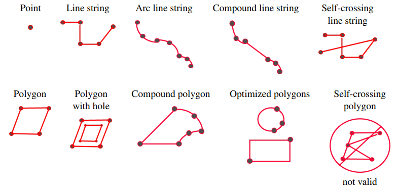
Point: represents point objects in 2, 3 or 4 dimensions.
Line: represents linear objects and is formed of straight lines or arcs. A closed line does not delineate a
surface and self-crossing lines are allowed. They are encoded as a list of points  .
.
Polygon: represents surface objects. The contour must be closed and the interior can contain one or more holes. The boundary cannot intersect and it is formed by straight lines or arcs (or a combination). Some specific forms as rectangles and circles can be expressed more efficiently.
An element is the basic component of geometric objects. The type of an element can be point, line or polygons. Fromed of an ordered sequence of points.
Represents a spatial object and is composed of an ordered list of elements, which may be homogeneous or heterogeneous.
Represents a geometrical column in a table. In general, it contains objects of the same nature.
Structure:
Example:
SDO_GTYPE
Define the nature of the geometric shape contained in the object.
SDO_SRID
SRID = Spatial Reference System ID. It specifies the coordinate system of the object. The list of possible values is in the table MDSYS.CS:SRS. A common value is 8307: which is ’Longitude/Latitude WGS84’, used by the GPS system. All geometries of a layer must have the same SRID. Layers may have different SRIDs. Automatic conversion for spatial queries.
SDO_POINT
Structure
Example
SDO_ORDINATES
Object type SDO_ORDINATE_ARRAY which is VARRAY (1048576) OF NUMBER. It stores the coordinates of lines and polygons.
SDO_ELEM_INFO
Object type SDO_ELEM_INFO_ARRAY which is VARRAY (1048576) OF NUMBER. It specifies the nature of the elements and describes the various components of a complex object. There three entries per element:
Ordinate offset: position of the first number for this element in the array SDO_ORDINATES.
Element type: type of the element.
Interpretation: straight line, arc,..
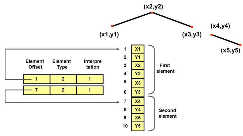
Examples of geometries:
Line:
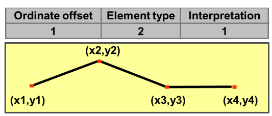
Polygon:
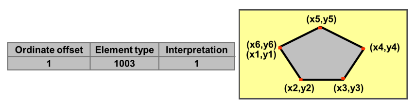
Multipoint:

Constructing a line
Metadata
Defines the boundaries of a layer, i.e., minimum and amximium coordinates for each dimension. Sets the tolerance of a layer, i.e., the maximum distance between two points for them to be considered different. And defines the coordinate system for a layer.
Example:
Constructing geometries
R-tree indexing: tree rectangles that provide indexing in 2 or 3 dimensions. It is based on the Minimum Bounding Rectangle (MBR) of objects.
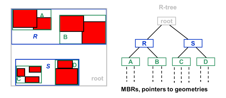
To create an index:
The CREATE INDEX statement may have additional parameters. To delete the index:
Quad-tree indexing: use a regular grid. It is not maintained in oracle now.
A spatial index must exists before we can ask spatial queries on a table.
But it can be optimized:
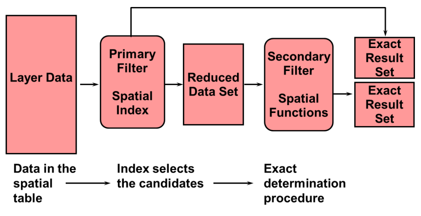
They contain a sptail predicate, and are expressed through specific SQL operators: SDO_RELATE, SDO_INSIDE, SDO_TOUCH, SDO_WITHIN_DISTANCE, SDO_NN. The spatial index must exists, otherwise we will get an error message.
Topological predicates
They select objects by their topological relationship with another object: SDO_INSIDE, SDO_CONTAINS, SDO_COVERS, SDO_COVEREDBY, SDO_OVERLAPS, SDO_TOUCH, SDO_EQUAL, SDO_ANYINTERACT.
The SDO_RELATE is a generic operator for which we can specify a mask, that can be ’INSIDE’, ’CONTAINS’, ’TOUCH’,... or a combination as ’INSIDE+CONTAINS’
Sample queries
Which parks are entirely contianed in the state of Wyoming:
Which states contain all or part of Yellowstone Park:
In which competing jurisdictions is my client:
Find all counties around Passaic County:
Queries with a constant window
Find all customers of type Platinum in a rectangular area:
In which competitor sales territories is located a geographical point:
Queries based on distance
These are used to select objects according to distance from another point. Distance can be expressed in any unit of distance and if no unit is specified, the distance is expressed in the unit of the coordinate system. For longitude/latitude data, these are meters. The function used is SDO_WITHIN_DISTANCE.
Which agencies are less than 1km form this client:
How many customers in each category are located within 1/4 mile of my office number 77:
Research based on proximity
These select the N closest objects of another objects: SDO_NN. ROWNUM can be used to limit result. SDO_NN_DISTANCE is used to categorize answers by distance.
What is the nearest office to this client?
What are my five customers closest to this competitor:
This only works if no other selection criterion is present.
What are my five customers closest to this competitor, and give the distance:
If we want to add more filters, we cannot use the SDO_NN function, because it is evaluated first. We have to do the trick with SDO_DISTANCE+ORDER BY+ROWNUM.
Spatial Join
It is used to find correlations between two tables, based on topology or distance. It compares all objects in a table with all those of another table, so it requires a R-Tree on each table. Technically implemented as a function that returns a table: the SDO_JOIN.
Associate with each GOLD customer the sales territory in which is is located:
Find all gold customers who are less than 500 meters from one of our branches in San Francisco:
Spatial functions
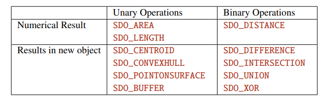
Objects must be in the same coordinate system.
What is the total area of Yellowstone National Park:
What is the length of the Mississippi riveer:
What is the distance between Los Angeles and San Francisco:
Generating objects
SDO_BUFFER(g,size) generates a buffer of the size chosen.
SDO_CENTROID(g) calculates the center of gravity of a polygon.
SDO_CONVEXHULL(g): generates the convex hull of the object.
SDO_MBR(g) generates the bulk of the rectangle object.
Combining objects
SDO_UNION(g1,g2)
SDO_INTERSECTION(g1,g2)
SDO_DIFFERENCE(g1,g2)
SDO_XOR(g1,g2) is the symmetric difference.
What is the area occupied by the Yellowstone Park in the state it occupies:
Spatial aggregation
Aggregate functions operate on the set of objects.
SDO_AGGR_MBR: returns the rectangle of space around a set of objects.
SDO_AGGR_UNION: computes the union of a set of geometric objects.
SDO_AGGR_CENTROID: calculates the centroid of a set of objects.
SDO_AGGR_CONVEXHULL: calculates the convex hull around a set of objects.
Find the focal point of all our customers in Daly City:
Calculate the number of customer in each zip code, and calculate the focal point for these clients:
 EmployeeTitle