Paper Review: Robust and Communication-Efficient Federated Learning from Non-IID Data

Introduction

This is a continuation post of the previous one, where we saw the paper Communication-Efficient Learning of Deep Networks from Decentralized Data.

In this post, we will see the paper Robust and Communication-Efficient Federated Learning from Non-IID Data, which proposes an enhancement to the Federated Averaging approach. In this paper, the authors propose a new compression method called Sparse Ternary Compression (STC), aiming to reduce the communication overhead of the Federated Averaging approach.

Motivation

One of the problems in FL settings is the communication overhead that arises from the several rounds of communication between the server and the clients, and the subsequent sending of the model from server to clients and vice versa. If comunication bandwidth is limited, FL can be inneficient or even unfeasible. The total amount of bits that need to be uploaded and downloaded by every client in the training process is given by: \[ b^{up/down} \in \mathcal{O}\left( N_{iter} \times f \times \left| \mathcal{W} \right| \times \left( H\left( \mathcal{W}^{up/down} \right) + \eta \right) \right), \] where:

• \(N_{iter}\) is the number of forward and backward passes per client in each round.
• \(f\) is the communication frequency.
  • \(N_{iter} \times f\) is the total number of updates per client.
• \(\left| \mathcal{W} \right|\) is the number of parameters in the model.
• \(H\left( \mathcal{W}^{up/down} \right)\) is the entropy of the weight updates exchanged during upload/download.
• \(\eta\) is the inefficiency of the encoding, i.e., the difference between update size and the minimal update size (the entropy).
  • \(\left| \mathcal{W}\right| \times H\left( \mathcal{W}^{up/down} \right) \times \eta\) is the total update size.

The authors consider the size of the model and the number of iterations per client as fixed, and focus on the three remaining factors:

• Reduce the communication frequency \(f\).
• Reduce the entropy of the updates \(H\left( \mathcal{W}^{up/down} \right)\) using lossy compression.
• Reduce the inefficiency of the encoding \(\eta\) using more efficient encoding schemes.

In addition, we have to consider the following challenges of the FL setting (see the previous post for more details):

• Unbalanced, non-IID data distribution.
• Large number of clients.
• Parameter server: it is common to use an intermediate parameter server to coordinate the training process. This reduces the amount of communication per client and communication rounds. However, it introduces a new challenge to communication-efficient training, since now both the upload to the server and the download from the server need to be compressed.
• Partial participation of clients: they can get out of battery or disconnected from the network.
• Small memory: the clients have limited memory, so it is necessary to keep the number of gradient evaluations per client low, as well as the batch size.

They conclude that a good method should fulfill the following requirements:

• R1: Compress both upstream and downstream communication.
• R2: Robust to non-IID data, small batch sizes and unbalanced data distribution.
• R3: Robust to partial participation of a great number of clients.

Limitations of Previous Compression Methods

Observe this figure, which shows the performance of different compression methods in the MNIST and CIFAR-10 dataset, with IID and non-IID data distribution, applying two different models (VGG-11 and Logistic Regression). In the non-IID case, there are two situations, in the first one (middle column), every client holds examples from two classes, and in the second one (right column), every client holds examples from only one class.

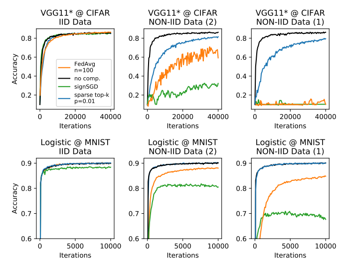
From this figure, we can conclude that:

• Federated Averaging (FedAvg): FedAvg suffers considerably from the non-IID data distribution, finding accuracy drops of up to 55% in non-IID environments as compared to IID ones.
• SignSGD: this is a quantization method that encodes only the direction of the gradient, and not its magnitude. As we can see in the figure, it performs even worse than FedAvg in the non-IID case.
• Top-k sparsification: this method keeps only the top-k largest gradients to be sent to the server. As depicted in the figure, it is the most robust method to non-IID data distribution, providing reliable convergence for both datasets.

Based on these observations, the authors provide two hypotheses:

1. The frequent communication between the server and the clients prevents them from diverging too much from one another.This is why top-k sparsification does not suffer from weight divergence, while FedAvg and SignSGD do.
2. Sparsification does not destibilize the training process as much as quantization does. This is why SignSGD performs worse than FedAvg.

However, top-k sparsification only compresses the upstream communication.

Therefore, the authors aimed at developing a new compression method that would be robust to non-IID data distribution, and that would compress both upstream and downstream communication.

Sparse Ternary Compression (STC)

Extension to downstream compression

Let \(\mathcal{W}\) be all the parameters of the model, \(W\) be one specific tensor of the model, and \(w\) be one specific element of the tensor \(W\).

Let

\[\begin{aligned}top_{p\%} & : & \mathbb{R}^n & \rightarrow & \mathbb{R}^n \\ & & \Delta\mathcal{W} & \mapsto & \Delta\hat{\mathcal{W}} \\ \end{aligned},\]

be the compression function that keeps only the \(p\) largest elements of \(\Delta\mathcal{W}\) and sets the rest to zero. Then, the update rule is:

\[\begin{aligned} \Delta\mathcal{W}^{t+1} = \frac{1}{n}\sum_{i=1}^{n}top_{p\%}\left(\Delta\mathcal{W}_i^{t+1}+A_i^t\right), \end{aligned}\]

where \(A_i^t\) is the residual, \(n\) is the number of clients and \(\Delta\hat{\mathcal{W}}_i^{t+1} = top_{p\%}\left(\Delta\mathcal{W}_i^{t+1}+A_i^t\right)\) is the compressed update from client \(i\). The residual can then be written as:

\[\begin{aligned} A_i^{t+1} = A_i^t + \Delta\mathcal{W}_i^{t+1} - \Delta\hat{\mathcal{W}}_i^{t+1}. \end{aligned}\]

Note that the client updates are always sparse, but the number of non-zero elements sent downstream in each round, \(\Delta\mathcal{W}_i^{t+1}\), grows linearly with the number of participating clients. If the participation rate is above the inverse sparsity, \(\frac{1}{p}\), this update is no longer sparse.

To solve this, the authors propose to use the same mechanism in the downstream communication, i.e., to keep only the \(p\) largest elements of \(\Delta\mathcal{W}^{t+1}\) and set the rest to zero. This is the Sparse Ternary Compression (STC) method. The update rule is:

\[\begin{aligned} \Delta\mathcal{W}^{t+1} = top_{p\%}\left(\frac{1}{n}\sum_{i=1}^{n}top_{p\%}\left(\Delta\mathcal{W}_i^{t+1}+A_i^t\right)\right) + A^t, \end{aligned}\]

with the server-side residual \(A^t\) defined as:

\[\begin{aligned} A^{t+1} = A^{t} + \Delta\mathcal{W}^{t+1} - \Delta\hat{\mathcal{W}}^{t+1}, \end{aligned}\]

where \(\Delta\hat{\mathcal{W}}^{t} = top_{p\%}\left(\Delta\mathcal{W}^{t}+A^{t-1}\right)\) is the compressed update from the server.

In the following figure, we observe how difference up and down sparsity levels affect the accuracy of the model:

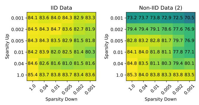
We observe how increasing the downstream sparsity level does not have very high impact on the accuracy when it’s of the same magnitude of the upstream sparsity level. This suggests that the downstream can be sparsified a bit more than the upstream without affecting the accuracy too much.

Weight Update Caching for Partial Client Participation

Next, the authors deal with the problem of keeping the clients synchronized, since they are not downloading the full model, but the sparse updates, and not all the clients participate in every round. To solve this, they propose a caching mechanism in the server.

Basically, if the last \(\tau\) rounds of updates, \(\{\Delta\hat{\mathcal{W}}^{t-\tau}, ..., \Delta\hat{\mathcal{W}}^{t-1}\}\), are cached in the server as a set of partial sums \({P^s = \sum_{t=1}^s \Delta\hat{\mathcal{W}}^t | s=1,…,\tau}\), as well as the global model \(\mathcal{W}^t\), then any client that wants to participate in the next round can do so by downloading some \(P^s\) or the global model, depending on how many rounds it has missed. The client can then compute the global model \(\mathcal{W}^t\) by adding the partial sums to the global model \(\mathcal{W}^t\).

Eliminating Redundancy

Finally, the authors try to increase the efficiency of the method, by eliminating the remaining sources of redundancy in the communication.

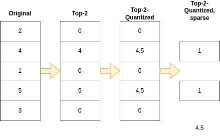
For this, they propose to combine sparsity with binarization. Instead of sending the top-\(k\) elements of the sparsified updates, they quantize them to \(\{-\mu, 0, \mu\}\), where \(\mu\) is the mean of the top-\(k\) elements. This is why the method is called Sparse Ternary Compression (STC).

In the next figure, we can see the effect of applying this quantization. It shows the accuracy of the model trained with only sparsity, minus the accuracy of the model trained with sparsity and quantization.

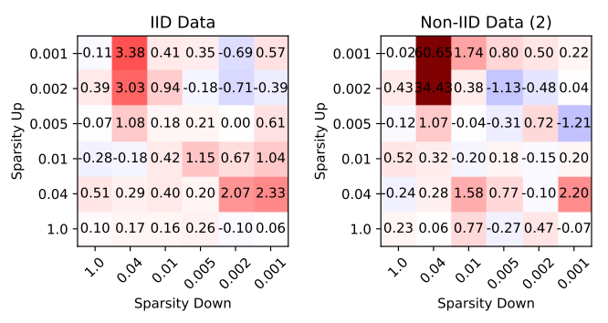
As we can see, the introduction of the quantization has a very small impact on the accuracy of the model in most cases, and in some cases it even improves it. This reassured the authors to include the quantization in the method.

In addition, they encode the sparse ternary updates using Golomb coding, which is a lossless compression method that provides statistical guarantees on the compression rate.

The process of the STC method for update compression is exemplified in the following figure:

Experiments

They did a good variety of experiments, using different models and datasets, and comparing the performance of the STC method with other compression methods. In this post, we will only focus on the most interesting ones.

They apply STC with the following parameters:

• Sparsity rate: \(p=\frac{1}{400}\)
• Delay period: \(n=400\)
• Number of clients: 100
• Participation ratio: 0.1
• Local batch size: 20

All methods used are given the same training budged, i.e., the same number of iterations per client and the same number of communication rounds.

Let’s delve into the different experiments.

Momentum in Federated Learning

Observe this Figure, where in the left plot every client hold data from exactly two different classes, while in the right plot every client holds an iid subset of data, and \(m=0.9\) is the momentum parameter:

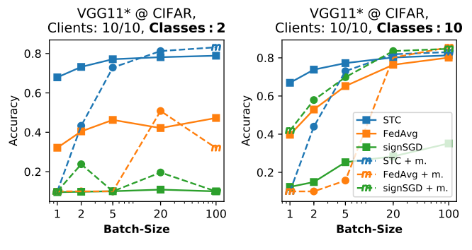
It shows how for increasing batch sizes, and for different amount of classes on the CIFAR dataset, STC remains stable, achieving good performance, while the other methods show a more unstable behavior.

In addition, it shows that if the participation rate is high, and the batch size is sufficiently large, momentum improves the performance of the model, while the opposite may happen if the participation rate is low and the batch size is small.

Different other graphs are shown in the paper, drawing a similar conclusion.

Robustness to Non-IID Data Distribution

Observe this Figure, where the accuracy is plotted against the number of classes per client, for different FL methods:

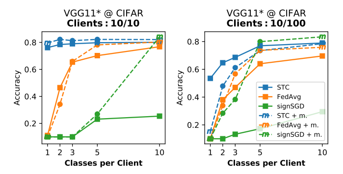
We observe how STC is the most robust method to non-IID data distribution (disregarding the use of momentum in some of the less non-iid setups), achieving the best performance in all cases. The difference is specially notorious when the data distribution is very non-IID, with only one or two classes per client.

Robustness to Partial Participation

Observe this Figure, where the accuracy is plotted against the participation rate, for different FL methods:

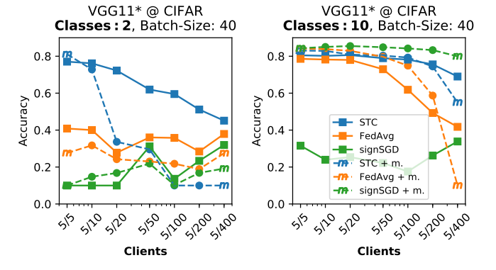
We can see how the decrease in participation rate has negative effects in both FedAvg and STC. However, STC still gets better results than FedAvg and SignSGD, even in the extreme case of using only 5 clients out of 400. The authors also mention that this is also not so bad, since the central server could increase the client participation if needed, at the expense of increased waiting time for all clients to finish their updates.

Conclusions

1. STC outperforms FedAvg and SignSGD, specially in non-IID environments, which are the most common in FL settings.
2. STC presents more advantages when the communication bandwidth is limited, since it compresses both upstream and downstream communication.
3. FedAvg should be used if the communication is latency-bound, since or if the client participation is very low and data is IID.
4. Momentum in FL should be avoided when data is highly non-IID, and when the participation rate is low and the batch size is small.

Basically, STC is a good alternative to FedAvg, specially in bandwidth-limited environments, and when the data distribution is non-IID. It is more robust to non-IID data distribution, and it compresses both upstream and downstream communication, which is a big advantage over FedAvg.