Neural networks

Introduction

In my previous post, I talked about perceptrons, which are the simplest neural networks. In this post, I will talk about multilayer perceptrons (MLP), which are one of the most commonly used neural networks and the easiest generalization of perceptrons.

For this, we will first see how we can use perceptrons to obtain multivariate outputs, basically by using multiple of them. Then, it will feel very natural to generalize this idea to obtain a multilayer perceptron. Finally, we will see how to train these networks using the backpropagation algorithm, which is an efficient algorithm to compute the gradient of a function which is a composition of other functions.

Using perceptrons for multiple outputs

We saw how to use a single perceptron to perform binary classification, and there is a very natural way to extend this model to multi-class classification, using a one-hot encoding for the class.

For instance, let’s work with a dataset \(\mathcal{D}=\left\{ x,y\right\} \), where \(x\in\mathbb{R}^{d}\) and \(y\in L=\left\{ l_{1},…,l_{K}\right\} \). We now encode \(y\) as a one-hot vector, i.e., \[y_{k}=\begin{cases} 0 & if\ y\neq l_{k}\\ 1 & if\ y=l_{k} \end{cases},\] for \(k=1,…,K\). The idea is then to use \(K\) perceptrons, each of them focusing on predicting one of the classes and trained independently. The idea is depicted in this figure: 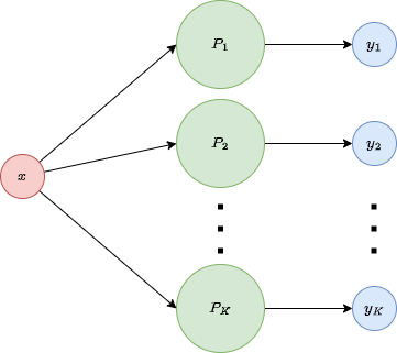Notice that in this case it is almost compulsory to use the logistic function (or a similar function, but definitely not the step function), since this way we can interpret the values as probabilities, and therefore select the value with highest probability as our prediction. Also, remember than in \(x\) we are adding an artificial 1 to account for the bias.

Let’s formalize this idea a little bit. We have \(K\) independent perceptrons, each of them predicting a variable, so that if we call \(g\) our activation function, we obtain, for each \(k=1,…,K\), \[ y_{k}\left(x\right)=g\left(w_{k}^{T}x\right), \] where \(w_{k}\) is the weight vector of perceptron \(k\). We can integrate all this into a single formula by introducing the notation \(f\left[\cdot\right]\),which applies \(f\) to each component of the input vector

\[f\left[x\right]=\left(\begin{array}{c} f\left(x_{1}\right)\\\\ \vdots\\\\ f\left(x_{d}\right) \end{array}\right).\]

This way, we can unify the previous equations as \[ y\left(x\right)=g\left[W^{T}x\right], \] where we have arranged

\[W=\left(\begin{array}{ccc} | & & |\\ w_{1} & ... & w_{K}\\ | & & | \end{array}\right).\]

Now, we can define what is a layer. A layer is just a set of parallel neurons and a layer with \(M\) neurons outputs \(M\) variables. Usually, all neurons in a layer use the same activation function,\(g\). Note that if this is not the case, then our previous explanation needs to be slightly adapted.

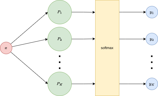
Since we have discussed that a good alternative in multiclass classification is to use the sigmoid function as activation function, we can rewrite our model as \[ y\left(x\right)=\sigma\left[W^{T}x\right]. \] Note, nonetheless, that here we are obtaining a bunch of different probabilities, one for each class, which could be further used to increase the information about our prediction. For instance, instead of computing the maximum out of these independent probabilities, we can add a softmax function to the outputs, resulting in a normalized vector that can now be considered as a probability vector. The softmax function is

\[y_k = softmax\left(z\right)_{k}=\frac{e^{z_{k}}}{\sum_{k'}e^{z_{k'}}}.\]

Also, when doing this, it is not necessary to apply the activation function, \(g\), beforehand. This approach is shown here:

Note that we are still in the linear classification scenario, and the next step is to improve the flexibility of the model to be able to cope with more complex relationships.

Multilayer perceptrons (MLP)

Notice now an interesting fact: if our activation function is \(g:\mathbb{R}\rightarrow I\), i.e., \(I\) is the range of \(g\), then a layer with \(M\) perceptrons can be interpreted as a function \[ G:\mathbb{R}^{n}\rightarrow I^{M}. \] For the sake of simplicity, let’s say \(G:\mathbb{R}^{n}\rightarrow\mathbb{R}^{M}\). Then, it is natural to think on stacking different layers, so that the output of a layers becomes the input of the following, effectively performing the composition of the functions defined by these layers.

For example, if we have two layers, which we interpret as two functions \(G^{\left(1\right)}:\mathbb{R}^{n}\rightarrow\mathbb{R}^{M_{1}}\) and \(G^{\left(2\right)}:\mathbb{R}^{M_{1}}\rightarrow\mathbb{R}^{M_{2}}\), we can take the output of the first layer and use it as input for the second one, effectively obtaining \[ G^{\left(2\right)}\circ G^{\left(1\right)}:\mathbb{R}^{n}\rightarrow\mathbb{R}^{M_{2}}. \] This is interesting mainly because a single layer, as we have seen, is only able to perform linear classification, but let’s delve a bit more on what is happening on the second layer. The second layer is using an activation function \(g^{\left(2\right)}:\mathbb{R}\rightarrow\mathbb{R}\), which is applied in each perceptron of the second layer as \[ y_{k}^{\left(2\right)}\left(x\right)=g_{k}^{\left(2\right)}\left(w_{k}^{\left(2\right)^{T}}\cdot y^{\left(1\right)}\left(x\right)\right)=g_{k}^{\left(2\right)}\left(w_{k}^{\left(2\right)^{T}}\cdot g^{\left(1\right)}\left[W^{\left(1\right)^{T}}\cdot x\right]\right). \] This means that we are:

• Creating $M_{1}$ combinations of the input variables, \(W^{\left(1\right)^{T}}\cdot x\), where \(W^{\left(1\right)}\in\mathcal{M}_{M_{1}\times\left(n+1\right)}\) (the \(+1\) is to account for the bias).
• Applying a different transformation \(g_{k}^{\left(1\right)}\) to each combination of variables. Note that this transformation can be arbitrary, but should be non-linear if we want to go out of the linear world, and should be differentiable if we want a smooth training process.
• For the second layer, the inputs are the transformations of the combinations of the input variables, which effectively become a base of functions (just as polynomials are), which are combined again by \(w_{k}^{\left(2\right)^{T}}\).
• Finally, we apply \(g_{k}^{\left(2\right)}\), which will be again an activation function.

The key steps for going beyond linearity are the second and third. Let’s compare it to a normal linear regression. In that case, basis functions can be introduced^{1 2} to be able to go out of the linearity world, by transforming the input variables. But then, we still use linear regression over this transformation. Therefore, it is the modification of the input what allows us to model non-linear relationship, and not the algorithm itself, which does not changed at all. Here, the idea is similar. In fact, we could just perform the same transformations that we used to in this new case, and keep applying just one layer of perceptrons to obtain non-linear classifiers. But this is exactly the power of the multi-layer perceptron: we don’t need to assume or guess the shape of the basis function! The different weights of the different layers will adapt to our problem, effectively auto-selecting how these functions should be. Of course, this is not free, and the cost is paid by obtaining harder trainings.

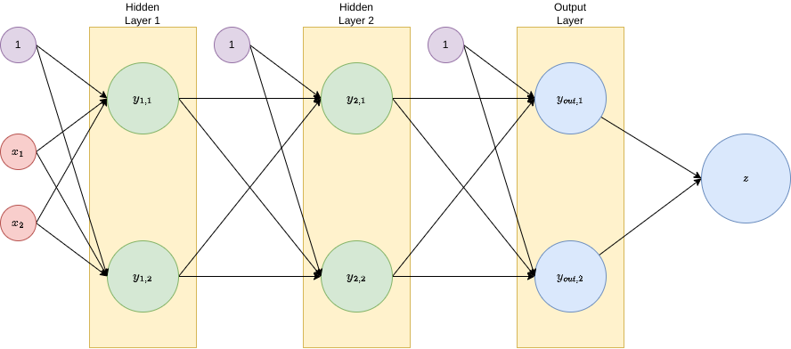
After this explanation, we can first integrate the previous formula as \[ y^{\left(2\right)}\left(x\right)=g^{\left(2\right)}\left[W^{\left(2\right)^{T}}\cdot g^{\left(1\right)}\left[W^{\left(1\right)^{T}}x\right]\right]. \] We can also define the multi-layer perceptron as composition of layers of perceptrons, with the addition of what is called the input layer, which is not really a layer of perceptrons, but rather represents and fixes the size of the input, and the output layer, which is the final layer, outputing the predictions of the model. The rest of the layers, the real perceptron layers, are called hidden layers. This is depicted the following figure:

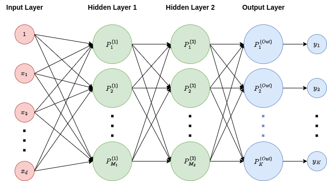
In this case, the first layer has \(M_{1}\) perceptrons, the second one has \(M_{2}\) perceptrons, and the output layer has as many perceptrons as possible labels, \(K\).

Observe that we have connected all outputs of each layer to all perceptrons in the second layer, also, note that two neurons within the same layer do not connect. These are just decisions and is not compulsory, and many different architectures exist.

More generally, a neural network is a directed graph whose nodes are perceptrons. If there are no cycles within the network, then it is a feed-forward neural network (FFNN), and it is called a recurrent network (RNN) in the case of cycles existing within the network.

MLP are thus a special case of feed-forward neural network, in which:

• Neurons are arranged in layers.
• There is at least one hidden layer.
• Every layer is fully connected to the next one.
• No connections are allowed within layers.

Backpropagation

Error function

The error in the regression case can be the empirical mean square error, i.e., \[ E\left(W\right)=\frac{1}{2}\sum_{i=1}^{n}\left(y_{i}-y_{W}\left(x_{i}\right)\right)^{2}, \] where the dataset is \(\left\{ \left(x_{i},y_{i}\right)\right\} _{i=1}^{n},y_{W}\left(x_{i}\right)\) is the prediction of \(x_{i}\) with the weight matrix \(W\). Note that in this formula we are assuming a single output, but it can be easily generalized as \[ E\left(W\right)=\frac{1}{2}\sum_{i=1}^{n}\left\Vert y_{i}-y_{W}\left(x_{i}\right)\right\Vert ^{2}. \] As usual in machine learning, our objective will be to minimize this error.

In the case of binary classification, if the target values are \(y_{i}\in\left\{ 0,1\right\}\), then we can express \[ P\left(y|x\right)=y_{W}\left(x\right)^{y}\left(1-y_{W}\left(x\right)\right)^{1-y}. \] If we assume independent and identically distributed examples, then we can define our likelihood function as \[ \mathcal{L}\left(W\right)=\prod_{i=1}^{n}y_{W}\left(x_{i}\right)^{y_{i}}\left(1-y_{W}\left(x_{i}\right)\right)^{1-y_{i}}, \] and the negative log-likelihood defines the cross-entropy error:

\[E\left(W\right)=-\log\mathcal{L}\left(W\right)=-\sum_{i=1}^{n}y_{i}\log\left(y_{W}\left(x_{i}\right)\right)+\left(1-y_{i}\right)\log\left(1-y_{W}\left(x_{i}\right)\right).\]

This formula can be generalized for multi-class classification, with \(K>2\) classes, as the generalized cross-entropy error: \[ E\left(W\right)=-\sum_{i=1}^{n}\sum_{k=1}^{K}y_{i,k}\log\left(y_{W,k}\left(x_{i}\right)\right). \]

Chain rule

Notice that the error functions that we have defined can be very complex, and there is no closed form solution to minimize them. Therefore, some iterative approach is necessary, as we did with the perceptron. But we encounter now a new problem: if we do gradient descent on the neural network, we will need to compute lots of gradients, and computing a gradient is not cheap. The idea to make this process more efficient is to use the chain rule and to notice that many of the gradients that we compute are actually used in many places along the network for the computation of the final gradient. Therefore, an improved version for computing gradients was developed: the \textbf{backpropagation algorithm}. This algorithm is based on the chain rule, and it is used to compute the gradient of the error function with respect to the weights of the network. Therefore, it is interesting to first review the chain rule.

The chain rule³ states that, given two composable differentiable functions \(f,g\), it is \[ \frac{d}{dx}f\left(g\left(x\right)\right)=f’\left(g\left(x\right)\right)\cdot g’\left(x\right). \] In the multivariate case, when we want to compute the derivative of \(f\left(g_{1}\left(x\right),...,g_{m}\left(x\right)\right)\), it is \[ \frac{d\left(f\left(g_{1}\left(x\right),…,g_{m}\left(x\right)\right)\right)}{dx}=\sum_{i=1}^{m}\frac{\partial f}{\partial y_{i}}\left(g_{1}\left(x\right),…,g_{m}\left(x\right)\right)\cdot\frac{dg_{i}}{dx}\left(x\right). \] This is sometimes written by naming \(z=f\left(g_{1}\left(x\right),...,g_{m}\left(x\right)\right)\) and \(y_{i}=g_{i}\left(x\right)\), so that the formula becomes (Notice the abuse of notation though.): \[ \frac{dz}{dx}=\sum_{i=1}^{m}\frac{dz}{dy_{i}}\frac{dy_{i}}{dx}. \]

Example

Let’s do an example to understand how this can be helpful in the case of neural networks.

Imagine we have the functions:

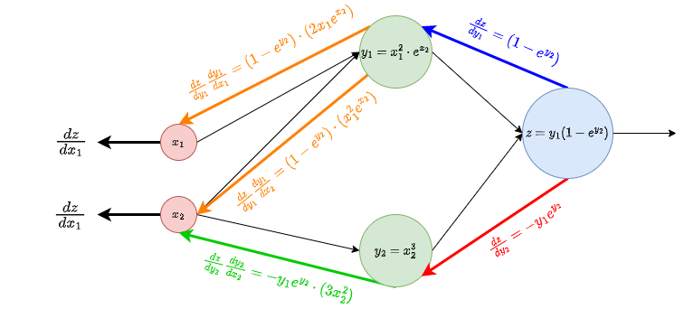
\[\begin{align*} y_{1} & =x_{1}^{2}\cdot e^{x_{2}}\\ y_{2} & =x_{2}^{3}\\ z= & y_{1}\left(1-e^{y_{2}}\right), \end{align*}\]

and we want to compute the gradient of \(z\) in terms of \(X\). We can write this as a diagram:

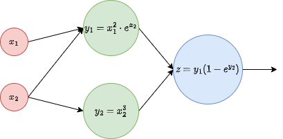
We simply need to compute the gradient using the chain rule:

\[\nabla z=\left(\begin{array}{c} \frac{dz}{dx_{1}}\\ \frac{dz}{dx_{2}} \end{array}\right)=\left(\begin{array}{c} {\frac{dz}{dy_{1}}}\frac{dy_{1}}{dx_{1}}+{\frac{dz}{dy_{2}}}\frac{dy_{2}}{dx_{1}}\\ {\frac{dz}{dy_{1}}}\frac{dy_{1}}{dx_{2}}+{\frac{dz}{dy_{2}}}\frac{dy_{2}}{dx_{2}} \end{array}\right)=\left(\begin{array}{c} {\left(1-e^{y_{2}}\right)}2x_{1}e^{x_{2}}-{y_{1}e^{y_{2}}}\cdot0\\ {\left(1-e^{y_{2}}\right)}x_{1}^{2}e^{x_{2}}-{y_{1}e^{y_{2}}}3x_{2}^{2} \end{array}\right)=\left(\begin{array}{c} {\left(1-e^{y_{2}}\right)}2x_{1}e^{x_{2}}\\ {\left(1-e^{y_{2}}\right)}x_{1}^{2}e^{x_{2}}-{y_{1}e^{y_{2}}}3x_{2}^{2} \end{array}\right).\]

Basically, the idea is to be able to reuse as many values as possible. To do this, we can compute local derivatives in each layer, and propagate them back to the previous layer, multiplying them. The previous computation can be done in the diagram as follows:

Note that:

1. We can avoid unnecessary computations by storing at each node:
   1. Forward values: when we evaluate \(y_{1}\left(x_{1},x_{2}\right)\), we can keep this value stored in the node, because we will need it later. In this example we did symbolic differentiation, so this was not necessary, but in neural networks we need to first to the forward pass, and then assess the error.
   2. Local derivatives: when we evaluate \(\frac{dy_{1}}{dx_{2}}\), we can keep this value stored in the node, because we will use it several times.
   3. Backwards gradients: local derivatives are sent to those nodes that will need them, so that each of this derivatives is computed only once. Then the gradient is constructed little by little, backwards, in a dynamic programming manner.
2. When the gradients are flowing backwards, each node has to sum all incoming gradients, according to the multivariate chain rule (if there is only one incoming gradient, we just take that one).

Backpropagation algorithm for neural networks

The pseudocode for backpropagation is as follows:

1. Forward pass
	- for layer in {1...c+1}
		a[layer] = W[layer]^T * z[layer-1]
		z[layer] = g[a[layer]] # apply g[.] to each component of a[layer]

2. Backward pass
	- d[c+1] = dg[a[c+1]] .* (z[c+1]-y) # .* is the component-wise product and dg is the derivative of g
	- grad[c+1] = z[c]*d[c+1]^T
	- for layer in {c...1}
		d[layer] = dg[a[layer]] .* (w[layer+1]*d[layer+1]) # w[k] is W[k] without the bias weigth
		grad[layer] = z[layer-1]*d[layer]^T

return grad

Let’s break it down.

• a[layer]=\(a^{\left(l\right)}\) is the input vector for layer \(l\).
• z[layer]=\(z^{\left(l\right)}\) is the output vector for layer \(l\), i.e., \(z^{\left(l\right)}=g_{l}\left[a^{\left(l\right)}\right]\), where \(g_{l}\) is the activation function of layer \(l\) (note in the pseudocode we are assuming the same \(g\) working on all layers).
• W[layer]=\(W^{\left(l\right)}\) is the weight matrix of layer \(l\).
• w[layer]=\(\hat{W}^{\left(l\right)}\) is the weight matrix of layer \(l\), without the weight of the bias.
• d[layer]=\(\delta^{\left(l\right)}\) is the local gradient at layer \(l\), computed as \[ \delta^{\left(out\right)}=g_{out}’\left[a^{\left(out\right)}\right]\odot\left(z^{\left(out\right)}-y\right) \] for the output layer, \(out\) or d[c+1] in the pseudocode, and \[ \delta^{\left(l\right)}=g_{l}’\left[a^{\left(l\right)}\right]\odot\left(\hat{W}^{\left(l\right)}\delta^{\left(l+1\right)}\right) \] for the rest of the layers, i.e., the hidden layers. Here, \(\odot\) is the Hadamard product, i.e., the component-wise product⁴. In the pseudocode, this is expressed by ‘.*’.

Example

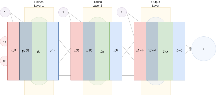
Let’s perform an example. Here is our neural network:

It is a fully connected two-layer network. Let’s follow the algorithm, defining each of the variables at a time.

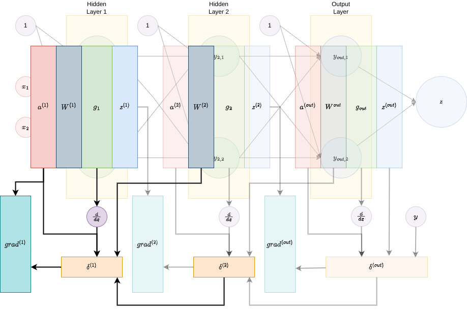
Forward pass. We define \(a^{\left(1\right)}=x,a^{\left(2\right)}=z^{\left(1\right)}=g_{1}\left[a^{\left(1\right)}\right],a^{\left(out\right)}=z^{\left(2\right)}=g_{2}\left[a^{2}\right]\) and \(z^{\left(out\right)}=z=g_{out}\left[a^{\left(out\right)}\right]\):

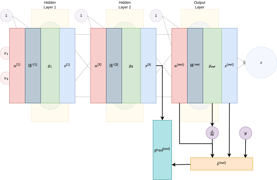
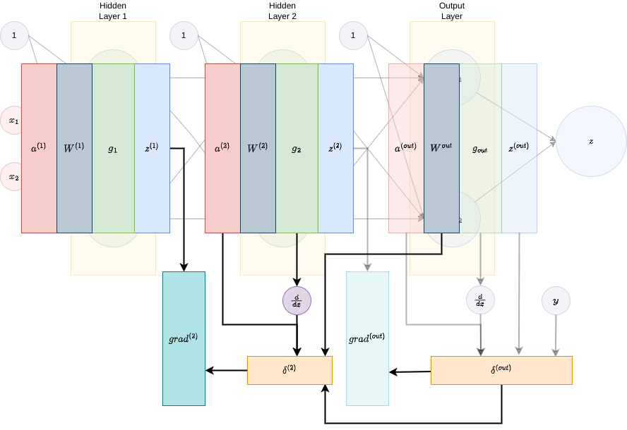
Backward pass.

• Step 0. Layer out (c+1). Define \(d^{\left(out\right)}=g_{out}'\left[a^{\left(out\right)}\right]\odot\left(z^{\left(out\right)}-y\right)\) and \(grad^{\left(out\right)}=z^{\left(2\right)}\cdot\delta^{\left(out\right)^{T}}\):

• Step 1. Layer 2. Define \(d^{\left(2\right)}=g_{2}'\left[a^{\left(2\right)}\right]\odot\left(\hat{W}^{\left(out\right)}\delta^{\left(out\right)}\right)\) and \(grad^{\left(2\right)}=z^{\left(1\right)}\delta^{\left(2\right)^{T}}\):

• Step 2. Layer 1. Define \(d^{\left(1\right)}=g_{1}'\left[a^{\left(1\right)}\right]\odot\left(\hat{W}^{\left(2\right)}\delta^{\left(2\right)}\right)\) and \(grad^{\left(1\right)}=z^{\left(0\right)}\delta^{\left(1\right)^{T}}=a^{\left(1\right)}\delta^{\left(1\right)^{T}}\):

And that’s it! Now we can use the gradient at each layer to train the network, updating the weights in layer \(l\) according to: \[ W^{\left(l\right)}=W^{\left(l\right)}-\gamma\cdot grad^{\left(l\right)}, \] where \(\gamma\) is the learning rate.

Activation functions

The logistic function is \(\sigma:\mathbb{R}\rightarrow\left(0,1\right)\), defined by \[ \sigma\left(x\right)=\frac{1}{1+e^{-x}} \] with derivative \[ \frac{d}{dx}\sigma\left(x\right)=\sigma\left(x\right)\left(1-\sigma\left(x\right)\right). \] In this case, for the backpropagation algorithm, we use \[ g’\left[a^{\left(l\right)}\right]=g\left[a^{\left(l\right)}\right]\odot\left(1-g\left[a^{\left(l\right)}\right]\right)=z^{\left(l\right)}\odot\left(1-z^{\left(l\right)}\right), \] which is a very efficient formula, since we have all this values computed in the forward pass.

The hyperbolic tangent function is \(tanh:\mathbb{R}\rightarrow\left(-1,1\right)\), defined by \[ tanh\left(x\right)=\frac{e^{x}-e^{-x}}{e^{x}+e^{-x}}, \] with derivative \[ \frac{d}{dx}tanh\left(x\right)=1-\left(tanh\left(x\right)\right)^{2}. \] Thus, we end up with another very efficient formula \[ g’\left[a^{\left(l\right)}\right]=1-z^{\left(l\right)}\odot z^{\left(l\right)}. \]

Conclusion

In this post we have set up the theoretical background for neural networks and the backpropagation algorithm. Of course, there are many considerations that we have not taken into account, such as the regularization, the optimization of the learning rate, the initialization of the weights, etc. However, this is a good starting point to understand the basics of neural networks.

In the next post we will see how to implement a neural network in Python or MATLAB (I will choose later, probably MATLAB), using the backpropagation algorithm.

I wish you have enjoyed the post :) If you have any question, comment or suggestion, please do not hesitate to contact me.

Bye!

References

1. There is a very brief and focused explanation in this notesonai’s post. ↩

2. You can check my notes on Machine Learning, UPC. ↩

3. For more information you can just visit Chain rule in Wikipedia ↩

4. For more information you can just visit Hadamard product in Wikipedia ↩