Implementing Neural Networks in MATLAB

Introduction

In the previous post, we saw how neural networks can be used for multi-class classification and the inners of the backpropagation algorithm for training them. In this post, we will see how to implement a neural network in MATLAB and train it using the backpropagation algorithm in the context of digit recognition.

The Dataset

The dataset we will use is the MNIST dataset¹, which contains 60,000 training images and 10,000 testing images of handwritten digits. Each image is a 28x28 grayscale image, which means that each image is represented by a 28x28 matrix of values between 0 and 255. The dataset is already split into training and testing sets, so we will use the training set for training and the testing set for testing:

load ('mnist.mat')

X_train = training.images;
Y_train = training.labels;
X_test = test.images;
Y_test = test.labels;

As an example, the following image is a 28x28 matrix representing the digit 8:

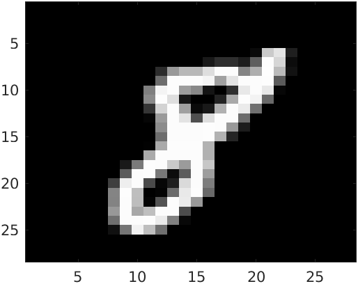
Note that the images are stored as a 28x28 matrix, but we will need to flatten them into a 784x1 vector in order to use them as input to the neural network. We will also need to convert the labels to one-hot vectors, which means that each label will be represented by a vector of length 10, where the index of the value 1 will be the digit represented by the image. For example, the digit 8 will be represented by the vector [0 0 0 0 0 0 0 0 1 0].

X_train = reshape(X_train,[784,60000])';
X_test = reshape(X_test,[784,10000])';

TT_train = Y_train + 1; % The function ind2vec needs positive values.
TTrain = full(ind2vec(TT_train'))';
TT_test = Y_test + 1;
TTest = full(ind2vec(TT_test'))';

The Model

Architecture and weights initialization

The input layer of the network has size 784, which is the number of the input images, as we have seen.

The output layer has size 10, since there are 10 possible digits (i.e., classes) that the network can predict.

Now, for the hidden layers, we need to make decisions. For this example, we are going to implement a network with a single hidden layer, of size 50.

inputLayerSize = 784;
hiddenLayer1Size = 50;
outputLayerSize = 10;

To initialize the weights, we can do the following:

function [W1, b1, Wout, bout] = generate_weights(input_size, layer1_size, output_size, scale)
    W1 = scale*(rand(layer1_size,input_size)-0.5);
    b1 = scale*(rand(layer1_size,1)-0.5);
    Wout = scale*(rand(output_size,layer1_size)-0.5);
    bout = scale*(rand(output_size,1)-0.5);
end

This function generates random weights for our network, with appropriate sizes. The weights are first generated between -0.5 and 0.5, and then multiplied by a scale factor.

The scale factor is needed because the weights are initialized randomly, and if they are too large, the network will not learn. If they are too small, the network will learn very slowly. The scale factor is a hyperparameter that we can tune to get the best results. You can tweak it to see what happens. For example, when I set it to 1, the networks predicts as a completely random classifier, and when I set it to 0.1, the networks works perfectly.

Now, we can initialize the weights:

[W1,b1,Wout,bout] = generate_weights(inputLayerSize,hiddenLayer1Size,outputLayerSize,0.1);

Activation functions

We will use the ReLU activation function² for the hidden layer, and the softmax activation function for the output layer. The ReLU function is defined as:

\[\text{ReLU}(x) = \max(0,x)\]

with derivative:

\[\text{ReLU}'(x) = \begin{cases} 0 & \text{if } x \leq 0 \\ 1 & \text{if } x > 0 \end{cases}\]

The softmax function is defined as:

\[\text{softmax}(x_i) = \frac{e^{x_i}}{\sum_{j=1}^n e^{x_j}}.\]

Note, however, that we will use the cross-entropy loss function, which is defined as³:

\[\text{cross-entropy}(y, z^{(out)}) = -\sum_{i=1}^n y_i \log(z^{(out)}_i)\]

And when we use the softmax function as the output activation function, the derivative of the cross-entropy loss function becomes very simple⁴:

\[\frac{\partial \text{cross-entropy}(y, z^{(out)})}{\partial z^{(out)}_i} = z^{(out)}_i - y_i.\]

So, we will not need to compute the derivative of the softmax function and the gradient of the cross-entropy loss function will be very cheap.

function ret = relu_func(z)
    ret = max(0,z);
end

function ret = relu_prime(z)
    ret = z>0;
end

function ret = softmax(z)
    ret = exp(z) ./ sum(exp(z),1);
end

Training

We have to define all the steps that we need to perform in order to train the network. We will use the following steps (notice that we are implementing exactly what was explained in the previous post):

1. Forward pass

function [A1,Z1,Aout,Zout] = forward_pass(X,W1,b1,Wout,bout)
    % X has the nrows records with ncols features
    A1 = W1*X'+repmat(b1,1,size(X,1));
    Z1 = relu_func(A1);

    Aout = Wout*Z1+repmat(bout,1,size(X,1));
    Zout = softmax(Aout);
end

1. Backward pass

function [grad_W1, grad_b1, grad_Wout, grad_bout] = backward_pass(Zout, T, Z1, X, Wout, A1)
    % Error in output
    d_output = Zout - T';

    % Gradient for output weights and biases
    grad_Wout = d_output * Z1';
    grad_bout = sum(d_output, 2);

    % Error in first layer
    d_layer1 = (Wout' * d_output) .* relu_prime(A1);

    % Gradient for first layer weights and biases
    grad_W1 = d_layer1 * X;
    grad_b1 = sum(d_layer1, 2);
end

1. Update weights

function [new_W1, new_b1, new_Wout, new_bout] = update_weights(lr,W1,b1,Wout,bout,grad_W1,grad_b1,grad_Wout,grad_bout)
    new_W1 = W1 - lr*grad_W1;
    new_b1 = b1 - lr*grad_b1;
    new_Wout = Wout - lr*grad_Wout;
    new_bout = bout - lr*grad_bout;
end

Now, everything is set up to train the network. We are going to train it using the algorithm called mini-batch gradient descent. This algorithm is very simple: we will split the training set into batches of size 100, and we will train the network using each batch. After each batch, we will update the weights of the network, using the backpropagation algorithm to compute the gradients. Every time we process the whole training set, we will say that we have completed an epoch. We will train the network for 20 epochs.

At the end of each batch, we use the network to predict the labels of the training set, and we compute the accuracy of the network. We will also compute the accuracy of the network on the test set, to see if the network is overfitting. For this computation, we defined the following function:

function accuracy = compute_accuracy(X, T, W1, b1, Wout, bout)
    % Feedforward
    [~, ~, ~, Zout] = forward_pass(X, W1, b1, Wout, bout);
    
    % Get the indices of the max values of the predicted and target labels
    [~, predicted_labels] = max(Zout);
    [~, true_labels] = max(T');
    
    % Compute accuracy
    accuracy = mean(predicted_labels == true_labels);
end

And finally, we can train the network:

learningRate = 0.01;
numEpochs = 20;
batchsize = 100;

accuracy_history = zeros(numEpochs, 1);

for epoch = 1:numEpochs 
    for i = 1:size(X_train, 1)/batchsize
        % Use the permuted indices to get the current example and label
        X = X_train(1+batchsize*(i-1):batchsize*i,:);
        T = TTrain(1+batchsize*(i-1):batchsize*i,:);
        
        % Feedforward
        [A1,Z1,Aout,Zout] = forward_pass(X,W1,b1,Wout,bout);
        
        % Backpropagation
        [grad_W1, grad_b1, grad_Wout, grad_bout] = backward_pass(Zout, T, Z1, X, Wout, A1);

        % Update weights and biases
        [W1, b1, Wout, bout] = update_weights(learningRate,W1,b1,Wout,bout,grad_W1,grad_b1,grad_Wout,grad_bout);
    end
    accuracy_history(epoch) = compute_accuracy(X_train, TTrain, W1, b1, Wout, bout);
    fprintf('Epoch %d: Accuracy: %0.5f\n', epoch, accuracy_history(epoch));
end

figure;
plot(1:numEpochs+1, accuracy_history);
title('Training Accuracy over Epochs');
xlabel('Epoch');
ylabel('Accuracy');

The output of the previous code is:

Epoch 1: Accuracy: 0.91012
Epoch 2: Accuracy: 0.94228
Epoch 3: Accuracy: 0.95607
Epoch 4: Accuracy: 0.96497
Epoch 5: Accuracy: 0.96605
Epoch 6: Accuracy: 0.96827
Epoch 7: Accuracy: 0.97248
Epoch 8: Accuracy: 0.97268
Epoch 9: Accuracy: 0.97395
Epoch 10: Accuracy: 0.97367
Epoch 11: Accuracy: 0.96990
Epoch 12: Accuracy: 0.97192
Epoch 13: Accuracy: 0.97407
Epoch 14: Accuracy: 0.97380
Epoch 15: Accuracy: 0.97337
Epoch 16: Accuracy: 0.97522
Epoch 17: Accuracy: 0.97515
Epoch 18: Accuracy: 0.97322
Epoch 19: Accuracy: 0.97260
Epoch 20: Accuracy: 0.97768

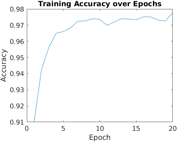
We can see how the accuracy is very good even after just one epoch. After 20 epochs, the accuracy is 97.3%, meaning the model predicts correctly most training examples. The following figure shows the accuracy of the network over the epochs:

Testing the model

Now, we can compute the accuracy of the model on the test set:

accuracy = compute_accuracy(X_test,TTest,W1,b1,Wout,bout);
fprintf('Accuracy: %0.5f\n', accuracy);

Which gives us:

Accuracy: 0.96180

The accuracy of the model on the test set is 96.2%, which is very good. This means that the model is not overfitting, and it is generalizing well to unseen data.

We can see some examples of the predictions of the model on the test set:

x = X_test(18,:);
pred = prediction(x,W1,b1,Wout,bout)
image (reshape(x*255,[28,28]));
colormap("gray")

The input image is:

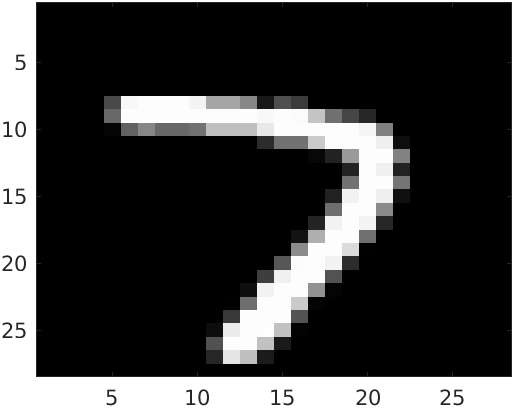
And the prediction of the model is 7, which is correct!

Two more examples input images that are correctly classified by the model:

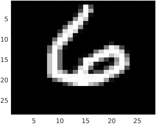
Is classified as a 4. And the following as a 6:

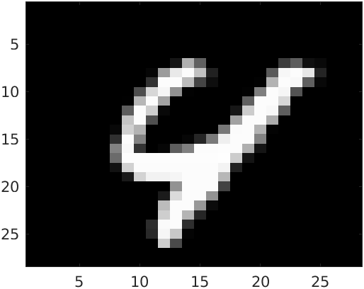
Of course, it is also interesting to see some examples of images that are not correctly classified by the model. For example, the following image is a 4, but the model classifies it as a 9:

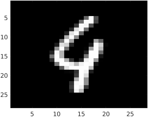
In defense of the model, I have to say that it is hard to say if it is a 4 or a 9.

Varying some parameters

In this section, we will see how the accuracy of the model changes when we vary some parameters. First, we will see how the accuracy changes when we vary the learning rate. We will use the following values for the learning rate: 0.001, 0.01, 0.1, 0.5, 1.0, 2.0, 5.0, 10.0. The following figure shows the accuracy of the model on the test set for each learning rate:

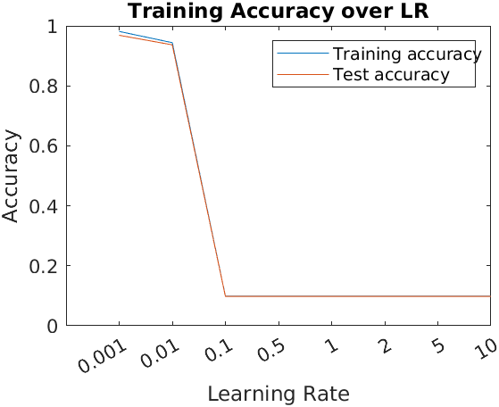
As we can see, the accuracy is maximized for the smallest learning rates, and from 0.1 on, the accuracy is just that of a random classifier. Note also that it remains constant from the third value on, which means that the model is not learning anything. This is because the learning rate is too big, and probably after a few interations, the weights and biases of the model are too big, and are too far away from the optimal values. This is a common problem in neural networks, and it is called the exploding gradient problem.

Another interesting variation is to see how the accuracy changes when we vary the number of hidden units. We will use the following values for the number of hidden units: 5,10, 20, 50, 100, 200, 500, 1000, 4000. The following figure shows the accuracy of the model on the test set for each number of hidden units:

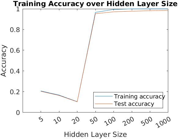
As can be observed in the plot, the training accuracy increases with the number of perceptrons used in the hidden units. However, this does not mean that the model is better, since it can be overfitting the training data. This is not the case this time, since in the plot we also observe that the accuracy on the test set is also increasing as well.

Nevertheless, take into account that the training time of the model also increases with the number of hidden units. In this case, the training time is not very big, but in more complex models, this can be a problem and is a factor to take into account.

Conclusions

In this post we have been able to implement a neural network to classify handwritten digits from the MNIST dataset, in MATLAB. We have been able to obtain a model that correctly classifies more than 95% of the images in the test set.

In addition, we have studied the behavior of the model when some parameters are varied, to get a deeper understanding of how each parameter affects the model. In particular, we have seen the importance of correctly selecting the learning rate, a decision that can make the model learn properly, or not learn at all. Also, how the number of hidden units affects the accuracy of the model as well as the training time.

I hope you liked the post and learnt something from it.

See you later!

References

1. Here, you can see an explanation on how to load the data to MATLAB: explanation. ↩

2. I did not define the ReLU function in the previous post, but you can consult ReLU in Wikipedia. ↩

3. You can see the derivation of the cross-entropy loss function in this post. ↩

4. I found this excelent post on softmax and cross-entropy that explains the softmax function and the cross-entropy loss function in detail. ↩