Classifiers in MATLAB

Theoretical background
Discriminant analysis is the result of implementing a Bayes classifier assuming that the class-conditional distributions \(p\left(x|y\right)\) are gaussian. This means that, having \(\mathcal{Y}=\left\{ c_{1},…,c_{K}\right\}\), then it is \[p\left(x|y=c_{k}\right)\sim\mathcal{N}\left(\mu_{k},\Sigma_{k}\right).\] If we also assume that the prior distributions are \[p\left(y=c_{k}\right)=\pi_{k},\] with \(\sum_{k}\pi_{k}=1\), then we define the discriminant functions \[g_{k}\left(x\right)=\log\left(P\left(y=c_{k}\right)P\left(x|y=x_{k}\right)\right)\] \[= \log\left(\pi_{k}\cdot\frac{1}{\det\left(\Sigma_{k}\right)^{\frac{1}{2}}\left(2\pi\right)^{\frac{d}{2}}}\exp\left\{ -\frac{1}{2}\left(x-\mu_{k}\right)^{T}\Sigma^{-1}\left(x-\mu_{k}\right)\right\} \right)\] \[= \log\pi_{k}-\frac{1}{2}\log\left(\det\Sigma_{k}\right)-\frac{d}{2}\log\left(2\pi\right)-\frac{1}{2}\left(x-\mu_{k}\right)^{T}\Sigma^{-1}\left(x-\mu_{k}\right)\] \[=\log\pi_{k}-\frac{1}{2}\left[\log\left(\det\Sigma_{k}+\left(x-\mu_{k}\right)^{T}\Sigma_{k}^{-1}\left(x-\mu_{k}\right)\right)\right]+const.\] This is a quadratic discriminant function, and the corresponding classifier is implemented by predicting \[ y’=c_{k’},\ where\ k’=\arg\max_{k}g_{k}\left(x\right).\] This corresponds to choosing the label with maximum probability a posteriori.
The decision boundaries in this case are those regions in which there exist \(k_{1},k_{2}\) with \[g_{k_{1}}\left(x\right)=g_{k_{2}}\left(x\right).\] These corresponds to hyper-quadrics in the feature space, and this is a quadratic method, usually called quadratic discriminant analysis (QDA).
Of course, we can further simplify our assumptions, by assuming that all labels have the same covariance matrix, \(\Sigma_{k}=\Sigma\) for all $k=1,…,K$. In this simpler case, the discriminant functions end up being \[g_{k}\left(x\right)=\log\pi_{k}+\mu_{k}^{T}\Sigma^{-1}x-\frac{1}{2}\mu_{k}^{T}\Sigma^{-1}\mu_{k},\] because now \(\det\Sigma_{k}=\det\Sigma\) is constant for all \(k\), so we can remove it. Furthermore, the term \(x^{T}\Sigma_{k}^{-1}x=x^{T}\Sigma^{-1}x\) is also constant with respect to \(k\), so it will not affect the \(k\) chosen. Therefore, we end up with linear discriminant functions, in which the decision boundaries correspond to hyperplanes in the feature space. This is a linear method, usually called linear discriminant analysis (LDA).
The nearest neighbor predictor uses the local neighborhood of an input point to compute a prediction. A well known family of this kind is the \(kNN\) models, which predicts the output of the input point by combining the known outputs of the \(k\) nearest training data points, for example by voting if we are classifying the data.
The approach of these method is quite straightforward, and is detailed in the following pseudocode:
Training
	Store all training examples

Prediction
	Given an input X:
		1. Compute distance/similarity with all examples in the training set.
		2. Locate k closest points.
		3. Emit prediction by combining outputs of the k closest points.
Of course, we have to decide:
- The distance/similarity function.
- How many neighbors to choose, \(k\).
- How to combine the outputs of the $k$ nearest neighbors to emit the final prediction.
Now, we are going to see how to use these methods in MATLAB.
LDA
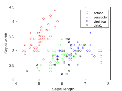
We are going to develop a classification example, using the famous Iris dataset.
load fisheriris
f = figure;
gscatter(meas(:,1), meas(:,2), species,'rgb','o',5);
xlabel('Sepal length');
ylabel('Sepal width');
We can perform LDA, to obtain a linear classifier:
lda = fitcdiscr(meas(:,1:2),species);
ldaClass = resubPredict(lda);

figure(f)
bad = ~strcmp(ldaClass,species);
hold on;
plot(meas(bad,1), meas(bad,2), 'kx');
hold off;
Now we can draw the regions:
figure;
[x,y] = meshgrid(4:.01:8,2:.01:4.5);
x = x(:);
y = y(:);
j = predict(lda, [x y]);
colors = [0 1 0; 1 0 0; 0 0 1];
face_alpha = 0.5;

% Loop through unique species and plot points with custom colors and transparency
unique_species = unique(j);
for i = 1:length(unique_species)
    scatter(x(strcmp(j, unique_species{i})), y(strcmp(j, unique_species{i})), [], colors(i,:), 'o', 'filled', 'MarkerFaceAlpha', face_alpha);
    hold on;
end
legend('versicolor','setosa','virginica')
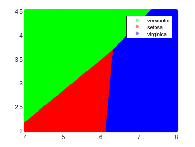
As we can see, the decision boundaries are hyperplanes (lines in the 2D case), which is a characteristic of linear classifiers.
QDA
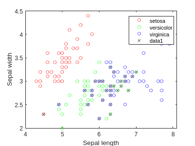
Let’s now repeat this with QDA, so that we can obtain non-linear regions:
f2 = figure;
gscatter(meas(:,1), meas(:,2), species,'rgb','o',5);
xlabel('Sepal length');
ylabel('Sepal width');

qda = fitcdiscr(meas(:,1:2),species,'DiscrimType','quadratic');
qdaClass = resubPredict(qda);

figure(f2)
bad = ~strcmp(qdaClass,species);
hold on;
plot(meas(bad,1), meas(bad,2), 'kx');
hold off;
figure;
[x2,y2] = meshgrid(4:.01:8,2:.01:4.5);
x2 = x2(:);
y2 = y2(:);
j2 = predict(qda, [x2 y2]);
% Define custom colors for the species
colors = [0 1 0; 1 0 0; 0 0 1];
face_alpha = 0.5;

% Loop through unique species and plot points with custom colors and transparency
unique_species = unique(j2);
for i = 1:length(unique_species)
    scatter(x2(strcmp(j2, unique_species{i})), y2(strcmp(j2, unique_species{i})), [], colors(i,:), 'o', 'filled', 'MarkerFaceAlpha', face_alpha);
    hold on;
end
legend('versicolor','setosa','virginica')
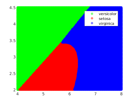
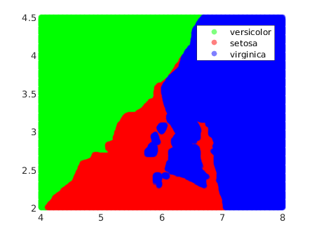
In this example we observe that the decision boundaries are no longer linear: they are quadrics in the input space. This fact increases highly the shapes that these boundaries can take.
For instance, a hyperplane is always ‘the same’, in the sense that all hyperplanes are isomorphic. On the other hand, quadrics are much more complex. In 2D, for example, these are the conics, which can take the form of a line, a ellipse (with the circunference as special case), a parabola or an hyperbola. This variety increases highly with the dimensionality. In 3D and above they are usually called quadrics, and in 3D there are 17 standard-form types [quadrics - wolfram mathworld].
kNN
A final example with a knn classifier:
% Train kNN classifier
k = 5; % You can change this value to choose a different number of neighbors
knn = fitcknn(meas(:,1:2), species, 'NumNeighbors', k);
knnClass = resubPredict(knn);

% Plot the dataset and misclassified points
f3 = figure;
gscatter(meas(:,1), meas(:,2), species, 'rgb', 'o', 5);
xlabel('Sepal length');
ylabel('Sepal width');

bad_knn = ~strcmp(knnClass, species);
hold on;
plot(meas(bad_knn, 1), meas(bad_knn, 2), 'kx');
hold off;

% Visualize the decision regions
figure;
[x3, y3] = meshgrid(4:.01:8, 2:.01:4.5);
x3 = x3(:);
y3 = y3(:);
j3 = predict(knn, [x3 y3]);

% Define custom colors for the species
colors = [0 1 0; 1 0 0; 0 0 1];
face_alpha = 0.5;

% Loop through unique species and plot points with custom colors and transparency
unique_species = unique(j3);
for i = 1:length(unique_species)
    scatter(x3(strcmp(j3, unique_species{i})), y3(strcmp(j3, unique_species{i})), [], colors(i,:), 'o', 'filled', 'MarkerFaceAlpha', face_alpha);
    hold on;
end
legend('versicolor','setosa','virginica')
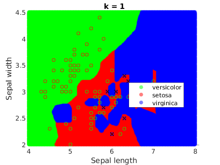
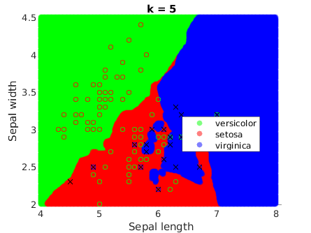
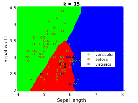
This method generates more complex decision boundaries, which are not even continuous. This is because kNN is not optimizing an underlying function, which is ultimately what creates the continuous boundaries that we have seen in the previous methods. In this case, the boundaries are highly determined by the data instances.
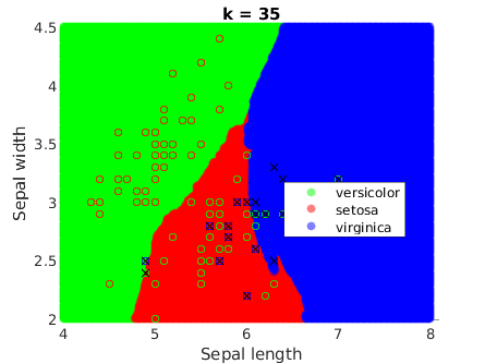
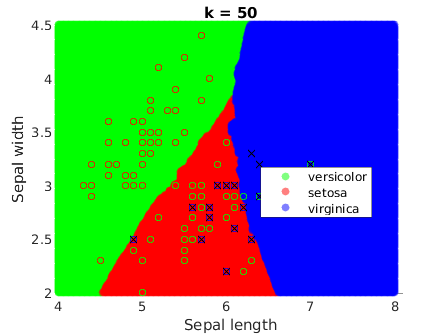
It is a remarkable fact that they get smoother when k increases:
load fisheriris

% Define custom colors for the species
colors = [0 1 0; 1 0 0; 0 0 1];
face_alpha = 0.5;

k_values = [1, 5, 15, 35, 50];

for k_idx = 1:length(k_values)
    k = k_values(k_idx);

    % Train kNN classifier
    knn = fitcknn(meas(:,1:2), species, 'NumNeighbors', k);
    knnClass = resubPredict(knn);

    % Visualize the decision regions
    f = figure;
    [x, y] = meshgrid(4:.01:8, 2:.01:4.5);
    x = x(:);
    y = y(:);
    j = predict(knn, [x y]);

    % Loop through unique species and plot points with custom colors and transparency
    unique_species = unique(j);
    for i = 1:length(unique_species)
        scatter(x(strcmp(j, unique_species{i})), y(strcmp(j, unique_species{i})), [], colors(i,:), 'o', 'filled', 'MarkerFaceAlpha', face_alpha);
        hold on;
    end

    % Plot the original dataset on top of the decision regions
    gscatter(meas(:,1), meas(:,2), species, 'rgb', 'o', 5);

    % Plot misclassified points
    bad_knn = ~strcmp(knnClass, species);
    plot(meas(bad_knn, 1), meas(bad_knn, 2), 'kx');

    hold off;

    % Set title and labels
    title(sprintf('k = %d', k));
    xlabel('Sepal length');
    ylabel('Sepal width');
    legend('versicolor','setosa','virginica')
end
Comparison
In this post, we explored three types of classifiers: Linear Discriminant Analysis (LDA), Quadratic Discriminant Analysis (QDA), and k-Nearest Neighbors (kNN).
LDA assumes that the different classes have the same covariance matrix. This leads to linear decision boundaries, making it a good choice when the classes are approximately normally distributed and have roughly the same covariance. It is also computationally efficient, which is beneficial when dealing with large datasets.
QDA, on the other hand, does not make the assumption of equal covariance matrices. This allows for more flexibility and can lead to better performance when the classes are normally distributed but have different covariances. However, QDA can be more sensitive to the estimation of the covariance matrix and may not perform as well when the number of features is large compared to the number of observations.
kNN is a non-parametric method that does not make any assumptions about the distribution of the classes. It can capture complex decision boundaries, but its performance can be heavily dependent on the choice of \(k\) (the number of neighbors) and the distance metric. It can also be computationally intensive for large datasets.
Conclusion
In conclusion, the choice of classifier depends on the specific characteristics of your data and the problem at hand. LDA and QDA are powerful tools when your data follows a Gaussian distribution, with LDA being more robust but less flexible than QDA. On the other hand, kNN can be a good choice when your data does not follow any specific distribution, or when the decision boundary is highly irregular.
Remember that these are just three of the many classifiers available. Other methods such as logistic regression, support vector machines, decision trees, and neural networks might be more suitable depending on your specific situation. Always consider the characteristics of your data and the assumptions of the method when choosing a classifier.
Finally, remember that you need to test your classifier and assess its performance on your specific problem.
I hope you liked the post and maybe even learned something new. Thanks for reading me!!11!1
References
- MATLAB fitdiscr documentation
- MATLAB fitcknn documentation
- MATLAB gscatter documentation
- You can check my notes on Machine Learning, UPC