Perceptron: The prelude of the neural networks

Introduction

We have all heard about neural networks, and how they are somehow a model of the human brain. Usually, this topic is presented as a black box, where we input some data, and we get some output. But, how does it work? What is the math behind it?

In this post I will try to explain what a perceptron is, both in plain words and in math. We will see how it works, and how it can be used to solve some problems. We will also see how it is related to neural networks. Finally, we will implement a perceptron from scratch in MATLAB.

What is a perceptron?

In the seek of understanding the behavior of the human brain, McCulloch and Pitts proposed in 1943 a model of a neuron, which they called a perceptron¹, later known as the McCulloch-Pitts neuron. This model is a simplified version of a real neuron, which they understood as a binary logic gate.

Let’s break this down a bit. I am not a biology guy, so forgive me if I am not accurate enough in this part. We all kind of know that there are 5 senses in our body, which basically gather information from our sorroundings. This information is then sent to the brain, where it is processed somehow, producing a response. This response is sent to different parts of the body, effectively producing an action, which can be conscious (moving your hand) or unconscious (breathing). The main mystery is how that processing is achieved. Ramón y Cajal discovered² that the brain is made of cells, which he called neurons. These neurons are connected to each other, and they are the ones that process the information. Information can be sent from one neuron to another through a synapse, which is basically a connection between two neurons. When a neuron receives enough information, it ‘fires’, sending signals to all the neurons to which it is connected. This is the basic idea of a neuron and what McCulloch and Pitts tried to model.

Here we can see a diagram of a neuron:

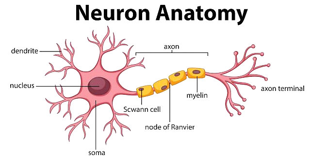
The neuron receives information from other neurons through the dendrites. This information is processed in the soma, and if it is enough, it fires through the axon, sending signals to other neurons through the synapses, which are the junctions between the axon terminals and the dendrites of other neurons.

Therefore, the neuron can be seen as a binary logic gate, which receives inputs and either produces an output or not. Mathematically, this writes as a function \[f:\mathbb{R}^n\rightarrow\{0,1\}\] where \(n\) is the number of inputs, and \(f\) is the activation function. This function can be defined in different ways, but the most intuitive one is to first perform a weighted sum of the inputs, and then apply a threshold function to the result. This approach is intuitive because the weighted sum is capturing the idea of the neuron being connected to other neurons, with different levels of importance, and the threshold function is capturing the idea of the neuron firing or not. Therefore, the activation function can be written as \[f(x)=\begin{cases}1&\text{if }w^Tx+b>0\\0&\text{otherwise}\end{cases}\] where \(x\in\mathbb{R}^n\) is the input, \(w\in\mathbb{R}^n\) is the weight vector, and \(b\in\mathbb{R}\) is the bias. The bias can be seen as the threshold of the neuron, and the weight vector as the importance of each input.

A visual representation of this function can be seen in the following figure:

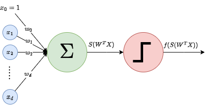
As we can see, the inputs are multiplied by the weights, and then added to the bias. If the result is greater than zero, the neuron fires, otherwise it doesn’t. Note that this is equivalent to a linear classifier, which separates the input space into two regions, one for each class. This is because the function is linear in the input, and therefore the decision boundary is a hyperplane.

Finding weights and bias

Now, how on Earth do we know the values of \(w\) and \(b\)? Well, this is the tricky part. We can’t just ask the neuron what are the values of \(w\) and \(b\), because it doesn’t know. We have to find them ourselves. This is done by training the neuron. The idea is to give the neuron some inputs for which we know what the output should be, and then adjust the values of \(w\) and \(b\) so that the output of the neuron is the expected one. This is done by using a loss function, which measures how far the output of the neuron is from the expected output. The loss function is usually defined as the squared error between the expected output and the actual output, that is \[L(w,b)=(y-f(x))^2,\] where \(y\) is the expected output. The idea is to minimize this loss function, so that the output of the neuron is as close as possible to the expected output. To minimize this value, we can try to just take the derivative of the loss function, and then set it to zero. However, this is not possible, because the loss function is not differentiable.

Therefore, a common approach is to change the activation function to a differentiable one, such as the sigmoid function, which is defined as \[\sigma(x)=\frac{1}{1+e^{-x}}.\] This function is differentiable, and it lies between 0 and 1, so that it can be interpreted as a probability of the neuron firing, instead of a binary output. This makes the model more flexible, as well as interpretable as a probability distribution, where the output variable is a Bernoulli random variable, \(y\sim Ber(\sigma(w^Tx+b))\). This is the approach that we will follow in this post. We can also embed the bias in the weight vector, by adding a 1 to the input vector, so that the perceptron function can be written as \[f(x)=\sigma(w^Tx).\] Now, instead of talking directly about error, it is more common to talk about the likelihood of the estimated model, which basically tells us how likely is the model to produce the observed data. The likelihood function is defined as \[\mathcal{L}(W)=\prod_{i=1}^m\sigma(w^Tx_i)^{y_i}(1-\sigma(w^Tx_i))^{1-y_i},\] where \(w={w_1,\dots,w_n}\) is the set of weights, \(x_i\) is the \(i\)-th input, and \(y_i\) is the \(i\)-th output. The idea is to maximize this function, so that the model is more likely to produce the observed data. This is equivalent to minimizing the negative log-likelihood, which is defined as \[-\log\mathcal{L}(W)=-\sum_{i=1}^m\left[y_i\log\sigma(w^Tx_i)+(1-y_i)\log(1-\sigma(w^Tx_i))\right].\] This function is called the cross-entropy loss function, and it is the one that we will use to train our perceptron.

When you differentiate it³, you get (after some computations): \[\nabla E(W)=\frac{\partial E(W)}{\partial W}=\sum_i[\sigma(w^Tx_i)-y_i]x_i.\] Unfortunately, this equation does not have a closed-form solution, so we have to use an iterative method to find the weights. The most common method is gradient descent, but other methods such as Newton’s method can also be used.

Gradient descent

Gradient descent is a general numerical method to find local minima of a differentiable function \(F(W)\). The idea is to use the fact that the gradient of a vector function points in the direction of maximum growth, and the negative gradient points in the direction of maximum decrease. Therefore, if we ’follow’ this direction, we should approach a minimum of the function, although it might not be the global minimum. The approach works as follows. To approximate a local minimum of \(F(W)\):

1. Initialize \(W_0\) to some random value. Set \(k=0\).
2. Compute the gradient of \(F(W)\) at \(W_k\), \(\nabla F(W_k)\).
3. Update \(W_k\) to \(W_{k+1}=W_k-\gamma\nabla F(W_k)\), where \(\gamma\) is the learning rate, and it quantifies ’how much’ we advance in the direction of the gradient. It has to be chosen beforehand and it is critical, since:
   • If \(\gamma\) is too small, the algorithm will take too long to converge.
   • If \(\gamma\) is too large, we might jump over the minimum and the method might never converge. Related to the learning rate is the importance of feature scaling, as the same learning rate impacts all features, so if they have different scales, the method might be good for some of them, but bad for others.
4. Repeat steps 2 and 3 until convergence.

Newton’s method

Newton’s algorithm⁴ is an algorithm used to find roots of a function which converges faster than gradient descent and does not need a learning rate parameter. As this algorithm finds roots (i.e. zeros), we don’t apply directly to \(F\) , but rather to its gradient. Thus, in this case, we need \(F\) to be twice differentiable and to be able to afford computing its second derivatives, which can sometimes be costly. In this case, the algorithm works as follows:

1. Initialize \(W_0\) to some random value. Set \(k=0\).
2. Compute the Hessian of \(F(W)\) at \(W_k\), \(H(F(W))=\nabla^2 F(W_k)\).
3. Update \(W_k\) to \(W_{k+1}=W_k-H(F(W_k))^{-1}\nabla F(W_k)\).
4. Repeat steps 2 and 3 until convergence.

When we apply Newton’s method to the perceptron, we are doing what is called Iterated Reweighted Least Squares (IRLS), and the Hessian is: \[H(F(W))=\nabla^2 F(W_k)=X^T\cdot diag(\sigma(w^Tx_i)(1-\sigma(w^Tx_i)))\cdot X.\]

Training the perceptron

Therefore, to train the perceptron, we give it examples \(X_i,y_i\) and we apply one of these methods to update the weights, according to the obtained result, for each example. This is called online learning, and it is the most common approach. The other approach is called batch learning, and it consists in applying the method to the whole dataset, instead of to each example.

Implementation in MATLAB

Step activation function

We are going to begin with an example using the step activation function, and then we will move to the sigmoid activation function. The learning algorithm is based on gradient descent, and you can consult it in my notes³ if you are interested in the details.

First, we generate the data that we want to classify. We want the model to be able to classify the points as 1 if they are bigger than 0.5, and as 0 otherwise. We will use the following code to generate the data:

rng(5)
X = rand([100,1]);
y = 2*(double(X>0.5)-0.5*ones(size(X)));

f=gscatter(X,zeros(size(X)),y,'br','o');
hold on
ylim([-0.1,0.1])
hold off

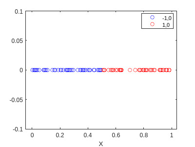
Now, this case is quite easy, and we can do it by hand. We know that the model is a line, and we can see that the line that separates the two classes is \(x=0.5\). Therefore, we can define the weights as \(w=[-0.5,1]^T\).

W = [-0.5; 1]

W = 2x1    
   -0.5000
    1.0000

If we use this model to classify the data, we get the following result:

% Add the bias
X_bias = [ones(size(X)) X];

pred = zeros(size(X));

for i=1:length(X)
    x = X_bias(i,:)';
    S = state(x,W);
    pred(i) = my_sign(S);
end

f2=gscatter(X,zeros(size(X)),pred,'br','o');
hold on
ylim([-0.1,0.1])
hold off

It classified perfectly! Now let’s train using the algorithm. First, we need to define the functions that we will need:

function S = state(X, W)
    S = W'*X;
end

function pred = my_sign(S)
    if S > 0
        pred = 1;
    else
        pred = -1;
    end
end

function W = train(X, y, lr, epochs)
    [~, d] = size(X);
    W = zeros(d, 1);
    for epoch = 1:epochs
        for i = 1:length(X)
            x = X(i,:)';
            pred = my_sign(state(x, W));
            if pred ~= y(i)
                W = W + lr*x*y(i);
            end
        end
    end
end

Now, we can train the model:

% Add the bias
X_bias = [ones(size(X)) X];

% Train the model
W2 = train(X_bias,y,0.1,10)

W2 = 2x1    
   -0.1000
    0.2013

pred2 = zeros(size(X_bias));

for i=1:length(X)
    x = X_bias(i,:)';
    S = state(x,W2);
    pred2(i) = my_sign(S);
end

f3=gscatter(X,zeros(size(X)),pred2,'br','o');
hold on
ylim([-0.1,0.1])
hold off

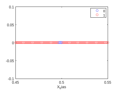
This is quite interesting… it found different weights, but it classified eveything well. This must break somewhere. Let’s try to determine where:

X = 0.45:0.001:0.55;
X = X';
y = 2*(double(X>0.5)-0.5*ones(size(X)));

X_bias = [ones(size(X)) X];

pred3 = zeros(size(X));

for i=1:length(X)
    x = X_bias(i,:)';
    S = state(x,W2);
    pred3(i) = my_sign(S);
end

f4=gscatter(X_bias,zeros(size(X)),pred3==y,'br','o');
hold on
ylim([-0.1,0.1])
xlim([0.45,0.55])
hold off

y(pred3~=y)

ans = 4x1    
    -1
    -1
    -1
    -1

This means that our model is actually setting the bound a little bit before 0.5 (as can be seen in the graph). This should be improved by increasing the size of X.

Sigmoid activation function

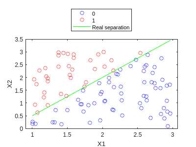
In this case, we will use a dataset a little bit more complex. We will generate the data using the following code:

rng(5)
X1 = rand([100,1])*2.+1;
X2 = rand([100,1])*3.;
y = double(X2>X1.*1.5-1);

X = [X1 X2];

f=gscatter(X1,X2,y,'br','o');
hold on
plot(X1,X1.*1.5-1,'g')
legend('0','1','Real separation','Location','northoutside')
hold off

Let’s train using gradient descent. Again, we define our training functions:

function S = state(X, W)
    S = X*W;
end

function s=logistic(S)
    s = 1./(1+exp(-S));
end

function ds=grad_logistic(y, y_hat, X)
    ds = X' * (y_hat - y);
end

function H = hess_logistic(y_hat, X)
    D = diag(y_hat .* (1 - y_hat));
    H = X' * D * X;
end

function [W,niter]=train_GD(X, y, lr, threshold, maxiter)
    [~, d] = size(X);
    W = ones(d, 1);
    for niter=1:maxiter
        st = state(X,W);
        y_hat = logistic(st);
        ds = grad_logistic(y, y_hat, X);
        v = vecnorm(abs(ds));
        if v < threshold
            break
        end
        W = W - lr*ds;
    end
end

function [W, niter] = train_NR(X, y, threshold, maxiter, lambda)
    [~, d] = size(X);
    W = ones(d, 1);
    I = eye(d);
    for niter = 1:maxiter
        st = state(X, W);
        y_hat = logistic(st);
        gradient = grad_logistic(y, y_hat, X);
        v = vecnorm(abs(gradient));
        if v < threshold
            break
        end
        H = hess_logistic(y_hat, X);
        W = W - inv(H + lambda * I) * gradient; %We add a term to avoid singularities
    end
end

function pred = my_predict(X, W)
    p = logistic(state(X, W));
    pred = double(p >= 0.5);
end

And we can now train the model:

[n, d] = size(X);
X_bias = [ones(n,1) X]; # Add the bias

[W,niter] = train_GD(X_bias,y,0.1,1e-3,20) #Train the model with learning rate 0.1, tolerance 1e-3 and 20 iterations

W = 3x1    
    3.9647
  -13.2924
   13.2435

niter = 20

And we can use our model to predict the output:

y_hat = my_predict(X_bias,W);

f2=gscatter(X1,X2,y_hat,'br','o');
hold on
plot(X1,X1.*1.5-1,'g')
legend('0','1','Real separation','Location','northoutside')
hold off

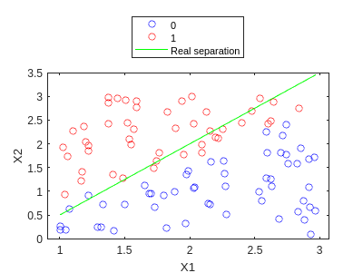
We can observe how it is quite ok… Let’s increment the max_iter parameters:

[W,niter] = train_GD(X_bias,y,0.1,1e-3,1000)

W = 3x1    
   20.9642
  -27.7530
   17.3205

niter = 1000

y_hat = my_predict(X_bias,W);

f3=gscatter(X1,X2,y_hat,'br','o');
hold on
plot(X1,X1.*1.5-1,'g')
legend('0','1','Real separation','Location','northoutside')
hold off

And in fact it is much better! :D

Let’s see how IRLS performs:

[W,niter_NR] = train_NR(X_bias,y,1e-3,1000,1e-3)

W = 3x1    
1.0e+05 *

    1.6554
   -2.0991
    1.2912

niter_NR = 227

y_hat = my_predict(X_bias,W);

f4=gscatter(X1,X2,y_hat,'br','o');
hold on
plot(X1,X1.*1.5-1,'g')
legend('0','1','Real separation','Location','northoutside')
hold off

We can see how this time we also obtain nice separation, and this one even finishes before maxiter is reached. In fact, we can try to see how many iterations would GD need:

[W,niter_GD] = train_GD(X_bias,y,0.1,1e-3,1000000)

W = 3x1    
  110.2037
 -146.6376
   92.3106

niter_GD = 449262

Therefore, we obtain an enormous speedup:

speedup = niter_GD / niter_NR

speedup = 1.9791e+03

Almost 2000 times faster in terms of iterations…

Conclusions

In this post we have understood the basics of the perceptron, and how it is useful to classify data. We have seen several methods to train it in the simple case of binary classification, and we have seen how IRLS needed much less iterations than GD to converge. Nonetheless, computing the Hessian can be quite expensive, and finding its inverse is not always possible.

We have seen how to implement the perceptron in Matlab, and how to train it using GD and IRLS, and even if the examples provided seems to be easy, you can change the data to whatever binary classification problem you want and it will work (note that this algorithms are not as optimized as the ones in Matlab, so they will be slower, but they will work).

I hope you learned something new, and if you have any question, feel free to ask me! In following posts we will see how to extend the perceptron to multiclass classification, and how to use it to solve regression problems. Then, we will be ready to see how perceptrons can be used to create neural networks, and how to train them using backpropagation.

See you in the next post!

References

1. McCulloch, W. S., & Pitts, W. (1943). A logical calculus of the ideas immanent in nervous activity. The bulletin of mathematical biophysics, 5, 115-133. ↩

2. Ramón y Cajal, S. (1894). The croonian lecture: La fine structure des centres nerveux. Proceedings of the Royal Society of London, 55, 444-468. ↩

3. You can check my notes on Machine Learning, UPC ↩ ↩²

4. There is an infinite amount of Newton’s algorithms haha, this is one of them :D ↩